How to Calculate the Inverse of a Matrix?

What is the Inverse of a Matrix?

Definition and Concept

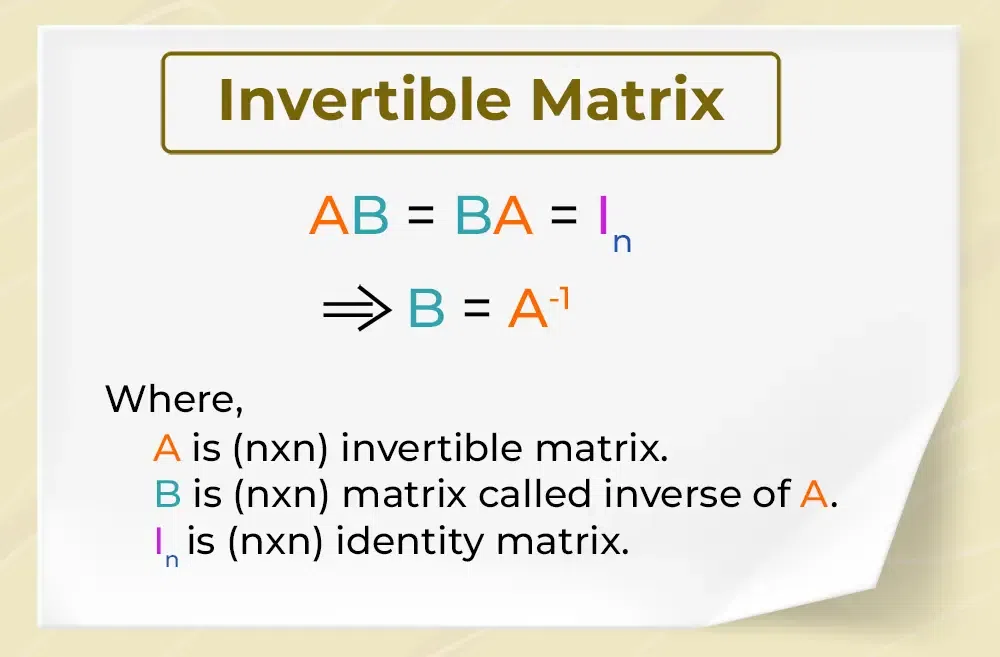
The inverse of a matrix is a concept that applies to square matrices (matrices where the number of rows equals the number of columns). The inverse of a square matrix \(A\) is denoted as \(A^{-1}\). If such a matrix exists, it satisfies the following property:

\(A \cdot A^{-1} = A^{-1} \cdot A = I\)

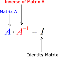
Where \(I\) is the identity matrix, a square matrix consisting of ones on its diagonal and zeros in all other entries. A matrix possessing an inverse is referred to as an invertible matrix or non-singular matrix. Matrices without inverses are termed singular matrices.

For example, consider a simple \(2×2\) matrix \(A = \begin{bmatrix} 1 & 2 \\ 3 & 4 \end{bmatrix}\). If \(A^{-1}\) exists, then multiplying \(A\) by its inverse will yield the \(2×2\) identity matrix \(I = \begin{bmatrix} 1 & 0 \\ 0 & 1 \end{bmatrix}\).

Identity Matrix and Conditions for Inverses

The identity matrix \(I\) is the fundamental element of matrix inversion. It serves the same role for matrix multiplication that the number \(1\) plays in scalar multiplication. For matrix \(A\), multiplication with \(I\) does not change \(A\):

\(A \cdot I = I \cdot A = A\)

Three essential conditions must be satisfied for a matrix inverse to exist:

1. The matrix must be square: Only square matrices (e.g., \(2×2\), \(3×3\), or \(n×n\)) are eligible for inversion. Non-square matrices, like \(2×3\), cannot have an inverse.

2.A matrix must have a nonzero determinant: this measure quantifies scalar properties within its square matrix structure. A matrix with zero or negative determinant properties is considered singular and doesn't possess an inverse matrix representation.

3. Matrices must possess full rank: This signifies that all rows (or columns, in matrix speak) of an array must be linearly independent from one another.

Common Methods to Calculate the Inverse of a Matrix

There are multiple methods to calculate the inverse of a square matrix, but the choice of method often depends on the matrix's size and its structure. Here, we focus on step-by-step procedures for \(2×2\) and \(3×3\) matrices and discuss general approaches for larger matrices.

Shortcut for \(2×2\) Matrices

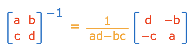
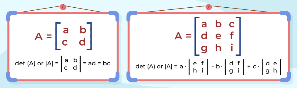
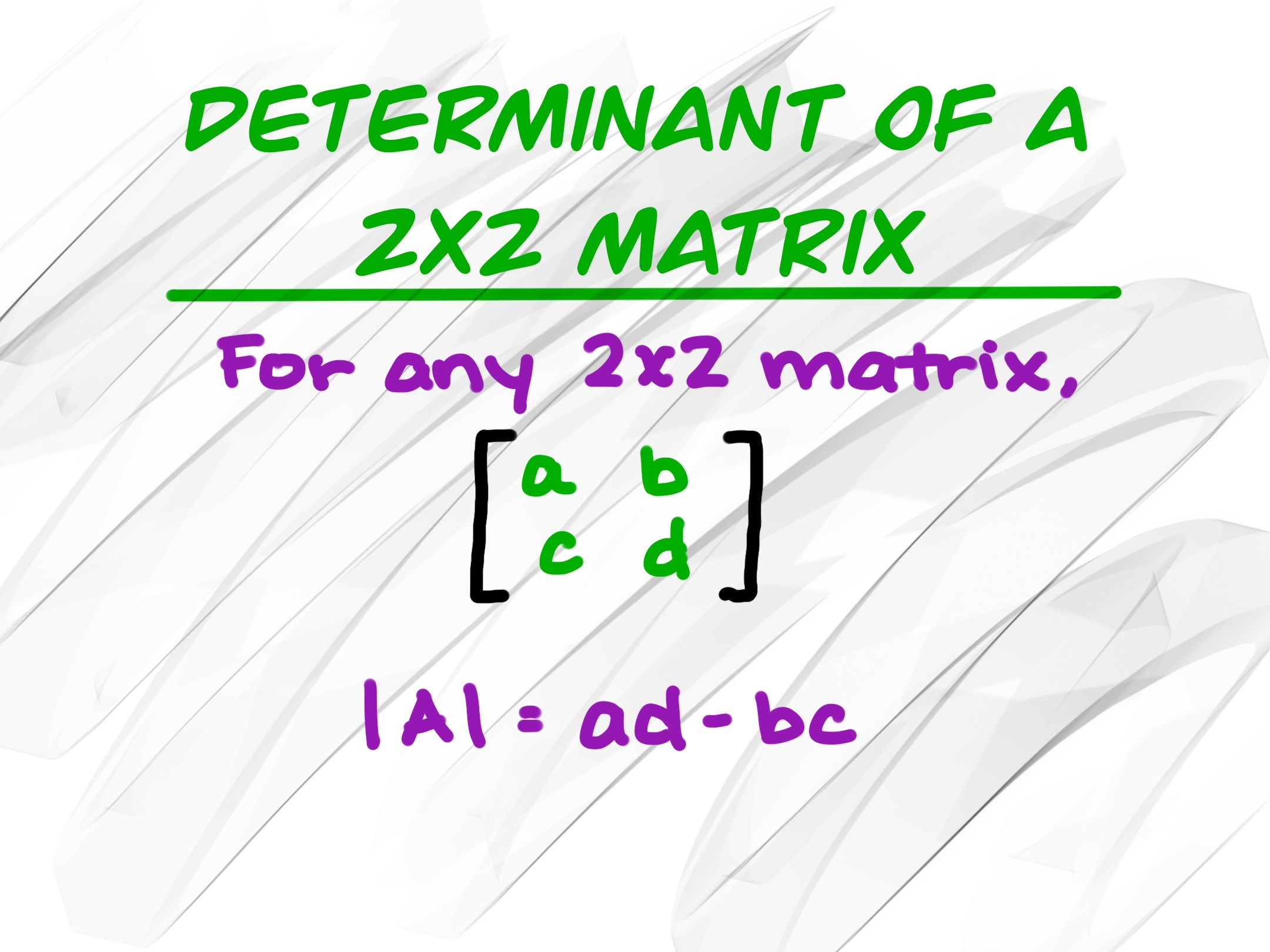
Finding the inverse of a \(2×2\) matrix is typically straightforward. Given a matrix \(A = \begin{bmatrix} a & b \\ c & d \end{bmatrix}\), its inverse \(A^{-1}\) exists only if the determinant is non-zero. The determinant (\(\text{det}(A)\)) is calculated as:

\(\text{det}(A) = ad - bc\)

The formula for the inverse of a \(2×2\) matrix is:

\(A^{-1} = \frac{1}{\text{det}(A)} \begin{bmatrix} d & -b \\ -c & a \end{bmatrix}\)

If \(\text{det}(A) = 0\), the matrix has no inverse.

Formula and Explanation

Using this formula, we can invert simple \(2×2\) matrices with ease. For example, let \(A = \begin{bmatrix} 2 & 1 \\ 5 & 3 \end{bmatrix}\).

1. Compute the determinant:

\(\text{det}(A) = (2)(3) - (5)(1) = 6 - 5 = 1\)

2. Substitute into the formula:

\(A^{-1} = \frac{1}{1} \begin{bmatrix} 3 & -1 \\ -5 & 2 \end{bmatrix} = \begin{bmatrix} 3 & -1 \\ -5 & 2 \end{bmatrix}\)

Real-World Usage

The \(2×2\) inversion formula is widely used in small systems such as basic mechanical systems, electrical engineering for impedance calculations, and economic models.

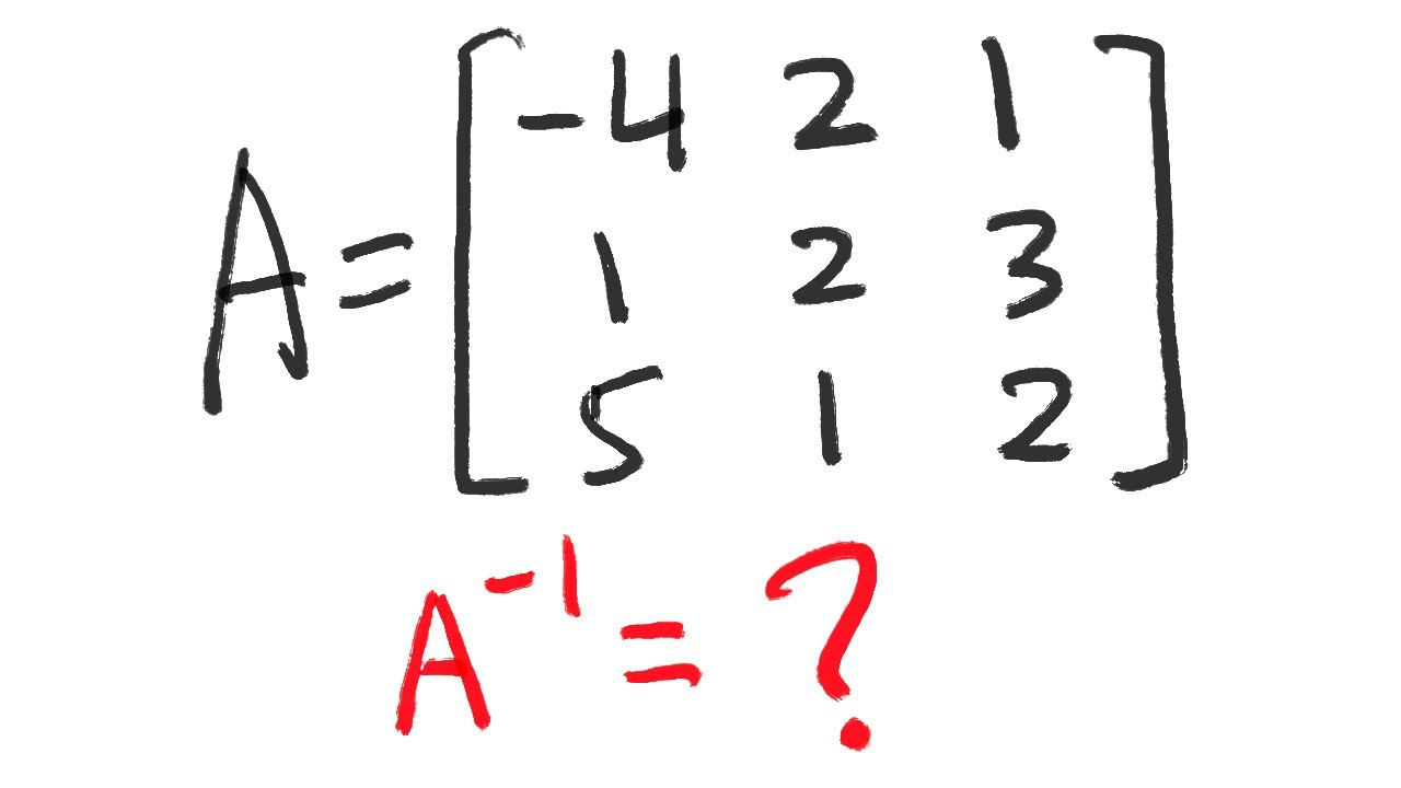
Inverse of \(3×3\) Matrices

The process for inverting a \(3×3\) matrix is more involved and consists of four main steps.

Step 1: Compute the Determinant

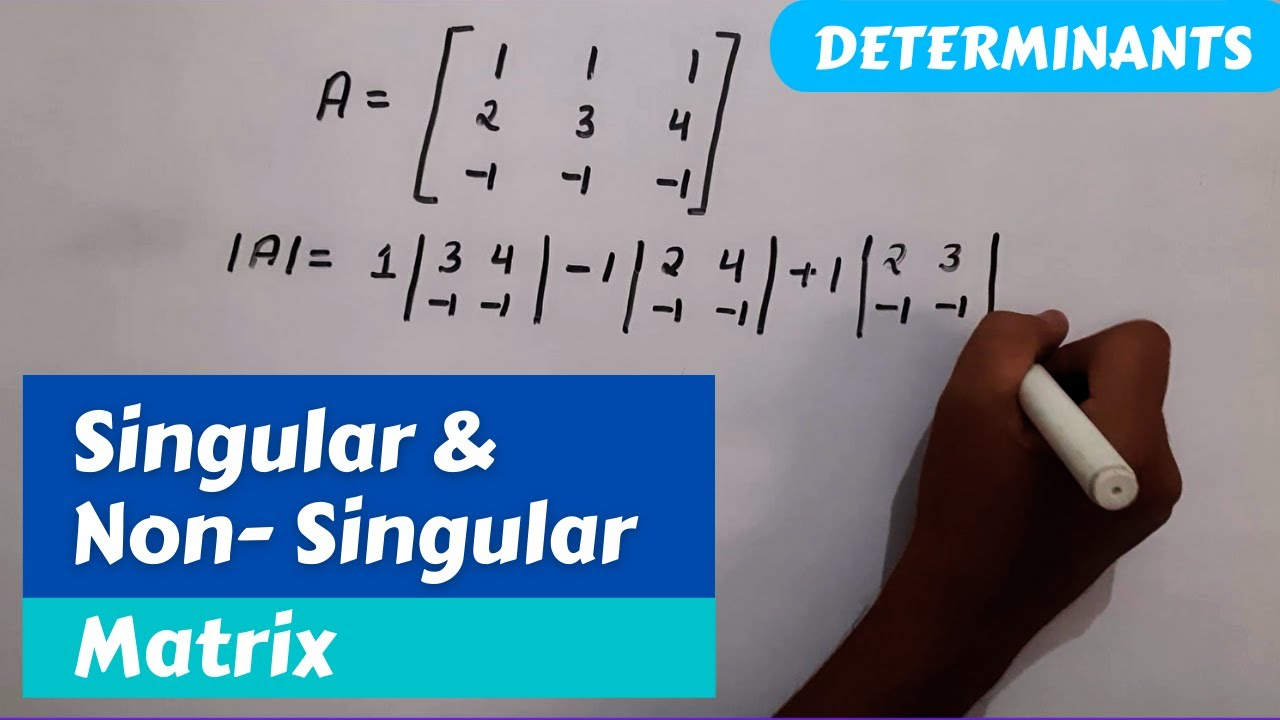
Given a \(3×3\) matrix \(A = \begin{bmatrix} a & b & c \\ d & e & f \\ g & h & i \end{bmatrix}\), the determinant is computed using:

\(\text{det}(A) = a(ei − fh) − b(di − fg) + c(dh − eg)\)

If \(\text{det}(A) = 0\), the matrix cannot be inverted.

Step 2: Calculate Minors & Cofactors

For each element \(a_{ij}\) of the matrix, calculate its minor by removing the \(i\)-th row and \(j\)-th column and computing the determinant of the remaining \(2×2\) matrix. The cofactor is the minor multiplied by \((-1)^{i+j}\).

For example, for \(A = \begin{bmatrix} 2 & 3 & 1 \\ 4 & 1 & 5 \\ 7 & 6 & 8 \end{bmatrix}\), the cofactor of \(a_{11}\) (2) is:

\(\text{Cofactor}(a_{11}) = (-1)^{1+1} \cdot \text{det}\begin{bmatrix} 1 & 5 \\ 6 & 8 \end{bmatrix} = (8 − 30) = -22\)

Step 3: Build the Adjoint Matrix

The adjoint of \(A\) is constructed by replacing each element of \(A\) with its cofactor and then transposing the resulting matrix.

Step 4: Use the Formula

Finally, the inverse is calculated as:

\(A^{-1} = \frac{1}{\text{det}(A)} \cdot \text{Adj}(A)\)

This step-by-step approach ensures precise computation for \(3×3\) matrices.

Elementary Row and Column Operations

Elementary row and column operations offer an efficient solution for matrix inversion. By appending an identity matrix to the right-side matrix and performing row-reducing operations, we transform both versions into equivalent identities while making both into inverted versions of themselves.

Steps to Invert a Matrix Using Augmentation

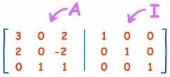
1. Form an augmented matrix: For \(A\), append the identity matrix \(I\) to form \([A | I]\).

2. Perform row-reduction: Use Gaussian elimination or row operations to transform \(A\) into \(I\). Apply the same operations to \(I\) simultaneously.

3. Read the result: Once \(A\) becomes \(I\), the modified \(I\) on the right becomes \(A^{-1}\).

This method is particularly useful for larger matrices and can be easily implemented in computational tools.

Scenarios Where This Method Is Useful

Row operations are especially useful when dealing with numerical solvers in computer programming or when a clear and systematic process is required for larger matrices.

Determinants and Their Role in Matrix Inversion

Determinants provide essential information about square matrices. Determinants play an essential part in deciding whether a matrix can be inverted since their properties directly link back to it.

Importance of Determinants

Determinants arise naturally during matrix operations such as solving systems of linear equations, deriving eigenvalues, and obtaining inverses.

When the determinant of a square matrix equals zero, its state is termed singularity, meaning it cannot be inverted into another matrix form.

For intuition, consider the geometric interpretation of determinants:

- In two dimensions (\(2×2\) matrices), the determinant corresponds to the area of the parallelogram formed by the column vectors of the matrix.

- In three dimensions (\(3×3\) matrices), the determinant indicates the volume of the parallelepiped defined by the column vectors.

When the determinant equals zero, the vectors are linearly dependent and collapse into a lower-dimensional space (e.g., a line or a point).

This explains why a singular matrix does not have an inverse.

Singular vs. Non-Singular Matrices

A singular matrix has a zero determinant and no invertible counterpart; by contrast, non-singular ones feature nonzero determinants, which allow inversion. Understanding why certain matrices do or do not possess inverses requires understanding this distinction between singular and non-singular matrix types.

For example:  

- Matrix \(B = \begin{bmatrix} 1 & 2 \\ 2 & 4 \end{bmatrix}\) is singular because its determinant is:  

\(\text{det}(B) = (1×4) - (2×2) = 4 - 4 = 0\)

This occurs because the rows (or columns) of \(B\) are linearly dependent.

- Matrix \(C = \begin{bmatrix} 2 & 1 \\ 3 & 4 \end{bmatrix}\) is non-singular because its determinant is:

\(\text{det}(C) = (2×4) - (1×3) = 8 - 3 = 5\)

Unique Properties of Determinants

Determinants can provide several useful properties that simplify matrix-related calculations:

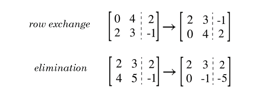
1. Effect of Row Swaps: Altering two rows (or columns) can alter its determinant. This change affects its sign and, thus, its calculation.

2. Row Add/Subtract Properties: Simply adding multiples from one row into another does not alter its determinant.

3. Scaling: Multiplying any row (or column) by an integer scales its determinant by that factor.

Utilizing these properties makes hand calculations faster.

Beyond \(3×3\) Matrices: Advanced Techniques

For matrices larger than \(3×3\), the computational effort required for inversion increases significantly. Advanced approaches, such as Gaussian elimination and exploiting special matrix structures, have become crucial.

Gaussian Elimination

Gaussian elimination is a systematic technique for solving systems of linear equations that can also be modified to find matrix inverses. The steps parallel those found in row-reduction methods discussed earlier:

1. Augment the matrix \(A\) with the identity matrix \(I\).

2. Apply row-reduction techniques to transform \(A\) into the identity matrix.

3. The transformed identity matrix becomes the inverse \(A^{-1}\).

For example, consider a \(4×4\) matrix \(D\). Gaussian elimination may involve hundreds of steps when conducted manually; however, with computers, it becomes much simpler. Gaussian elimination has proven to be an efficient and scalable computational method that is ideal for computational tasks.

Special Cases: Diagonal and Orthogonal Matrices

Certain categories of matrices, including diagonal and orthogonal matrices, possess special properties that make inversion easier.

Diagonal Matrices

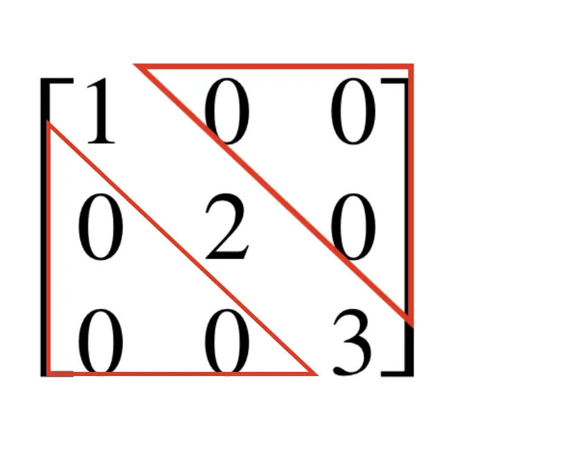
A diagonal matrix refers to a square matrix where all non-diagonal elements are zero. For example,

\(D = \begin{bmatrix} 3 & 0 & 0 \\ 0 & 7 & 0 \\ 0 & 0 & 5 \end{bmatrix}\)

The inverse of a diagonal matrix \((D)\) is calculated by taking the reciprocal of its diagonal elements:

\(D^{-1} = \begin{bmatrix} 1/3 & 0 & 0 \\ 0 & 1/7 & 0 \\ 0 & 0 & 1/5 \end{bmatrix}\)

Orthogonal Matrices

An orthogonal matrix \(Q\) is a square matrix whose rows and columns are orthonormal vectors. These matrices satisfy the property:

\(Q^{-1} = Q^T\)

This makes their inversion computationally inexpensive compared to general matrices.

Creative Approach: Visualizing Matrix Inverses through Graph Theory

Matrices can sometimes be illustrated and understood using other areas of mathematics such as graph theory - this nontraditional approach provides useful intuition for newcomers starting out.

Connecting Matrices and Graphs

Consider a graph \(G\), where the adjacency matrix \(A\) represents the connections between nodes. The inverse of \(A\), when it exists, can be seen as encoding indirect relationships or dependencies between nodes in the graph.

For instance, in a social network graph where nodes represent individuals and edges represent friendships, the inverse adjacency matrix could represent indirect trust relationships between people.

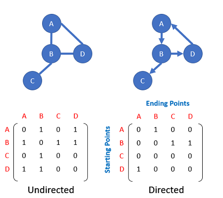
Beginner-Friendly Example of Graph Theory

Imagine a small network described by the \(2×2\) matrix \(A = \begin{bmatrix} 1 & 1 \\ 1 & 2 \end{bmatrix}\). Its inverse:

\(A^{-1} = \begin{bmatrix} 2 & -1 \\ -1 & 1 \end{bmatrix}\)

Has entries that reflect weighted relationships between the nodes, adjusted by the network's structure. While this is an abstract concept, tying matrix inverses to real-world systems like networks can aid understanding.

Tips and Tricks for Faster Calculations

Speeding up matrix inversions can involve understanding shortcuts as well as leveraging technology. Below, we share some practical tips.

Memorization Techniques for Small Matrices

For \(2×2\) matrices, memorizing the formula for inversion is sufficient. For slightly larger matrices (\(3×3\) specifically), practice calculating minors and cofactors to internalize the process.

Verifying Solutions Quickly

After computing the inverse, verify your result by multiplying the matrix \(A\) by its inverse \(A^{-1}\). The product should yield the identity matrix \(I\).

For example:

\(A = \begin{bmatrix} 1 & 2 \\ 3 & 4 \end{bmatrix}, \quad A^{-1} = \begin{bmatrix} -2 & 1 \\ 1.5 & -0.5 \end{bmatrix}\)

Check by multiplying:

\(A \cdot A^{-1} = \begin{bmatrix} 1 & 0 \\ 0 & 1 \end{bmatrix}\)

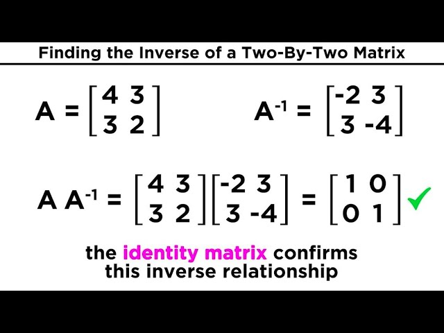
This step avoids propagating errors into subsequent calculations.

Real-World Applications of Matrix Inversion

Matrix inversion has critical applications in numerous domains. Below, we outline three key areas where it plays a vital role.

Science – Solving Systems of Equations

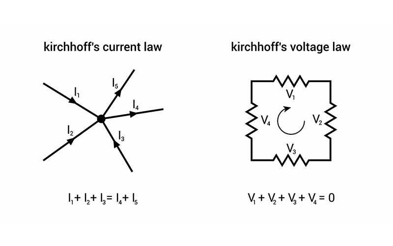
Matrix inversion is widely employed across physics and chemistry to solve systems of linear equations, for instance, in electrical circuit analysis when Kirchhoff's laws create equations in matrix form that need to be solved using inverting matrix forms; its use allows unidentified currents and voltages to be calculated more precisely; similarly in quantum mechanics when solving Schrödinger equation usually includes employing matrix inversion to predict particle wavefunctions as well as their probability distributions.

Engineering – Control and Stability

Engineering uses matrix inversion as an essential technique in both control theory and mechanical system analysis. Robotics rely on this practice for solving their inverse kinematics problems using matrix inversion; similarly vibration analysis employs stiffness/mass matrices inversion to evaluate system responses to dynamic forces for maximum design efficiency and system stability.

Statistics/Machine Learning – Optimization and Modeling

Statistics uses covariance matrices that have been inverted using Gaussian discriminant analysis or Mahalanobis distance calculations to establish relationships among variables, while machine learning relies on inversion for optimizing problems such as refining weights for regression or neural network training; matrix inversion accelerates convergence toward optimal parameters in high-dimensional spaces.

These applications demonstrate how matrix inversion can help solve complex issues across scientific, engineering, and computational fields.

Final Words: Choosing the Right Method

The choice of method for inverting a matrix depends on its size, structure, and context. Computational tools like MATLAB, Python’s NumPy library, and Wolfram Mathematica can expedite the process.

Recap of Methods Discussed

This article walked through shortcut methods for \(2×2\) matrices, step-by-step calculations for \(3×3\) matrices, computational tools for larger matrices, and the unique properties of special matrices.

Importance of Foundational Understanding

While software can quickly compute matrix inverses, understanding the mathematical process is key to diagnosing errors, optimizing code, and applying these concepts effectively.

Conclusion

Matrix inversion is an indispensable topic that spans mathematics, engineering, physics, computer science, and beyond. Computing and understanding inverse matrices is at the core of solving real-world issues ranging from electrical circuit analysis and robot motion optimization in engineering to performing statistical analyses supporting machine learning models and performing statistical analyses supporting machine learning models. Whether it's inverting a simple \(2×2\) matrix or dealing with large-scale matrices in advanced computations, mastering these techniques provides invaluable problem-solving tools.

Matrix inversion stands out as an exceptional way of simplifying and providing structured solutions to complex systems of equations. Not only is matrix inversion useful in terms of computational convenience, but understanding its underlying theory also deepens our grasp of key mathematical principles like determinants, linear independence, and matrix transformations - improving application accuracy while broadening our capacity to innovate new mathematical tools that adapt quickly to meet new challenges.

The software has made inverting matrices faster and more accessible; however, having a solid theoretical background enables practitioners to verify results, troubleshoot errors, and select methods appropriate to specific problems more quickly and confidently. Mastery of matrix inversion thus becomes not simply technical expertise but an opportunity to enhance critical thinking abilities as well as mathematical insight, which are important skills in both academic and professional environments.

Reference:

https://mathresearch.utsa.edu/wiki/index.php?title=The_Geometric_Interpretation_of_the_Determinant

https://chem.libretexts.org/Courses/Grinnell_College/CHM_364%3A_Physical_Chemistry_2_(Grinnell_College)/03%3A_The_Schrodinger_Equation_and_a_Particle_in_a_Box/3.04%3A_Wavefunctions_Have_a_Probabilistic_Interpretation

https://www.neuralconcept.com/post/the-role-of-structural-dynamic-analysis-in-engineering-design