How to Diagonalize a Matrix: A Comprehensive Guide

What is Matrix Diagonalization?

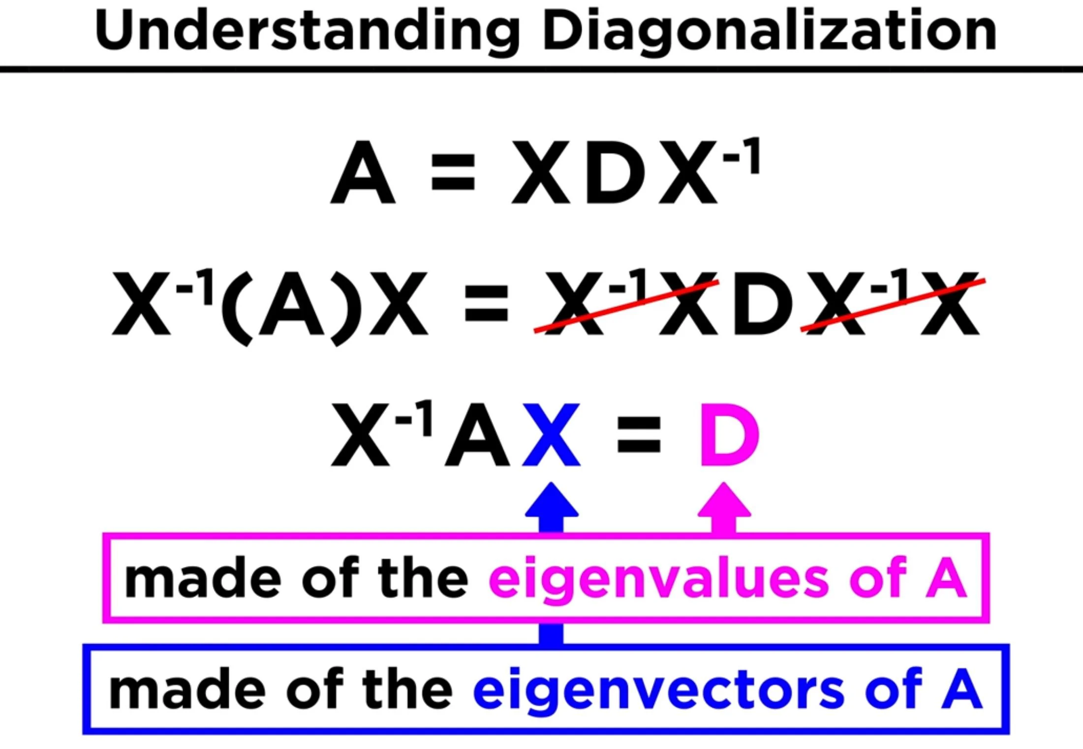
Diagonalization is the process of simplifying a square matrix by transforming it into a diagonal matrix, where all the off-diagonal elements become zero. A matrix \(A\) is diagonalizable if there exists an invertible matrix \(S\) and a diagonal matrix \(D\) such that \(S^{-1}AS = D\). The diagonal elements of \(D\) are the eigenvalues of \(A\), and the columns of \(S\) are the eigenvectors of \(A\). This technique is immensely useful in linear algebra because diagonal matrices are simpler to work with, as operations like matrix powers and exponentials become straightforward.

Matrix diagonalization plays an essential part in many applications, from solving systems of linear differential equations and mechanical system analyses, to decreasing computational complexity for data science algorithms. By understanding diagonalization techniques, students and professionals alike can uncover elegant yet efficient means of manipulating matrices to address real world issues more efficiently.

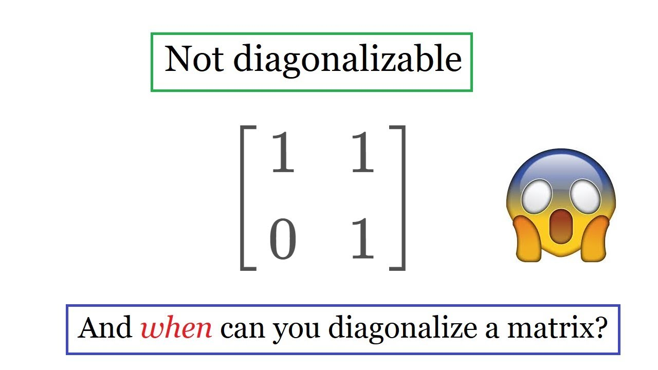
When Can a Matrix Be Diagonalized?

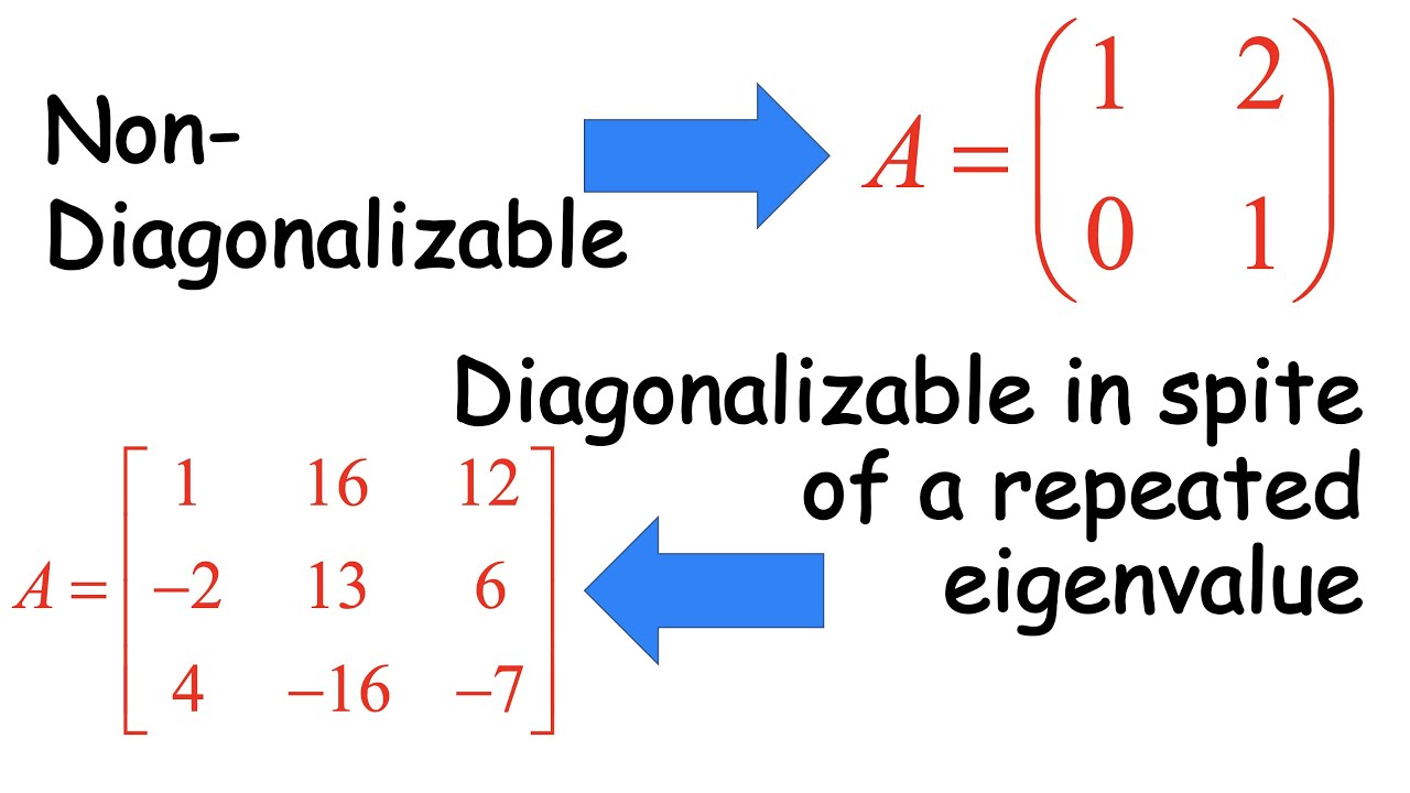
Not all matrices can be diagonalized. In order to be diagonalizable, a matrix must have enough linearly independent eigenvectors spanning its space in an effective fashion - specifically matching its geometric multiplicity (i.e., dimension of its eigenspace) with its algebraic multiplicity (number of times its value appears as roots in characteristic polynomials) precisely; otherwise known as defective matrices they cannot be diagonalized.

Matrices with distinct eigenvalues can always be diagonalized; however, those containing repeated eigenvalues may or may not meet this condition depending on the eigenspaces they occupy; defective square matrices cannot meet such conditions for diagonalization.

Key Concepts Behind Diagonalization

Eigenvalues and Eigenvectors

The concepts of eigenvalues and eigenvectors lie at the heart of matrix diagonalization.

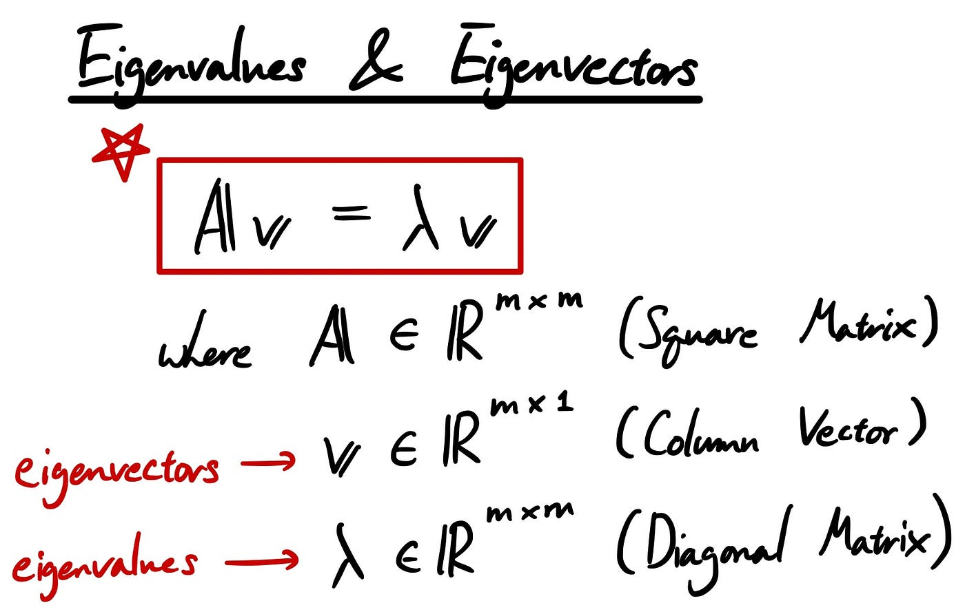
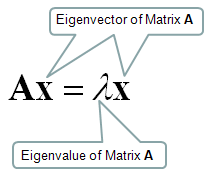
- Eigenvalues: If a matrix \(A\) acts on a vector \(v\), and the result is a scalar multiple of \(v\), then \(v\) is called an eigenvector, and the scalar \(\lambda\) is called the eigenvalue. Formally:

\(Av = \lambda v\)

Rearranging gives \((A - \lambda I)v = 0\), where \(I\) is the identity matrix. Finding eigenvalues requires solving the characteristic equation, \(\text{det}(A - \lambda I) = 0\), which provides the eigenvalues as the roots of the determinant equation.

- Eigenvectors: For each eigenvalue \(\lambda\), its eigenvectors lie in the null space (kernel) of \(A - \lambda I\). These eigenvectors define "directions" along which the linear transformation \(A\) stretches or compresses vectors by a factor of \(\lambda\).

Illustrative Analogy: Imagine stretching a spring in various directions until certain directions experience stretching or compression without altering their orientation; these are known as eigenvectors, and their amounts constitute their eigenvalues; mechanical engineers often utilize this concept when studying stress or vibration analysis, while in machine learning Principal Component Analysis (PCA) relies upon them for data variance determination.

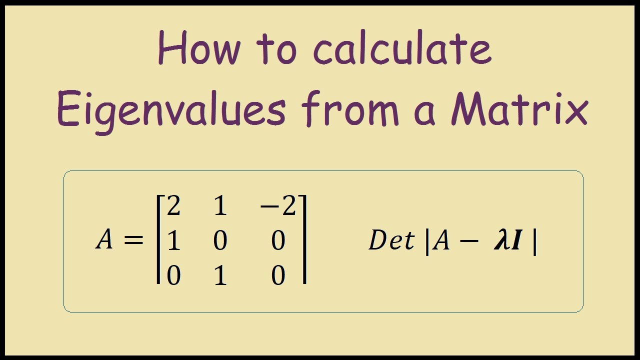
Characteristic Polynomial and its Role

To diagonalize a matrix \(A\), you must first compute its eigenvalues by solving the characteristic polynomial:

\(p(t) = \text{det}(A - tI)\)

Here, \(A - tI\) refers to the matrix \(A\), where \(t\) acts as a placeholder for eigenvalues along the diagonal of the identity matrix \(I\). The determinant gives a polynomial equation, and solving \(p(t) = 0\) yields the eigenvalues of \(A\).

- Algebraic Multiplicity: This is the number of times a root (eigenvalue) appears in \(p(t)\).

- Geometric Multiplicity: This represents the dimension of the eigenspace or the number of linearly independent eigenvectors associated with a particular eigenvalue.

For diagonalization, the essential condition is that geometric multiplicity = algebraic multiplicity for all eigenvalues. If this condition is not satisfied, the matrix is defective and cannot be diagonalized.

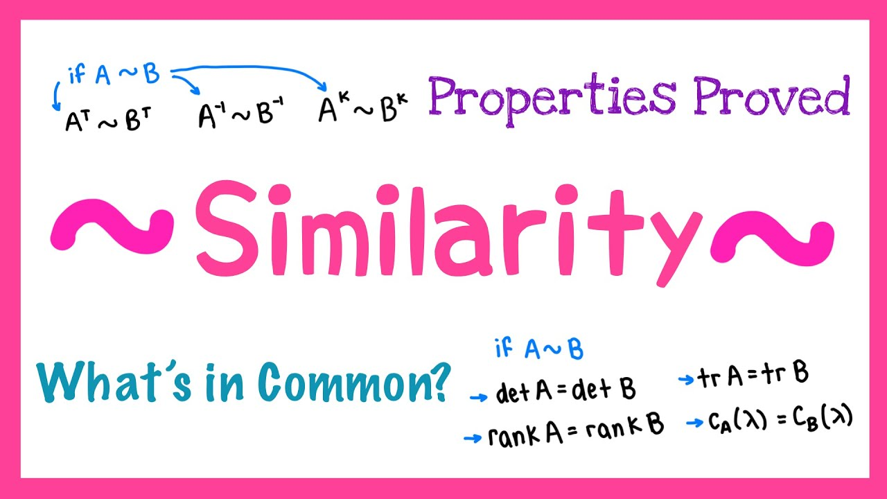
Similarity Transformations

Matrix diagonalization relies on the concept of similarity transformations. Two matrices \(A\) and \(B\) are said to be similar if there exists an invertible matrix \(S\) such that:

\(B = S^{-1}AS\)

In the case of diagonalization, \(B\) becomes the diagonal matrix \(D\), and \(S\) contains the eigenvectors of \(A\) as its columns.

Properties Retained Under Similarity Transformations:

- Determinant

- Trace (sum of the diagonal elements)

- Rank

- Eigenvalues (but not eigenvectors)

Investigation of similarity is critical because the eigenvalue decomposition \(S^{-1}AS = D\) forms the theoretical basis of diagonalization.

Step-by-Step Process of Diagonalizing a Matrix

Step 1 - Find the Characteristic Polynomial

The first step in diagonalizing a matrix is to compute its eigenvalues using the characteristic polynomial:

\(p(t) = \text{det}(A - tI)\)

1. Construct \(A - tI\) by subtracting \(t\) from the diagonal entries of \(A\).

2. Compute the determinant of \(A - tI\).

Example: For \(A = \begin{bmatrix} 2 & 3 \\ 1 & 4 \end{bmatrix}\),

\(A - tI = \begin{bmatrix} 2 - t & 3 \\ 1 & 4 - t \end{bmatrix}\)

\(p(t) = \text{det}(A - tI) = (2 - t)(4 - t) - (3)(1) = t^2 - 6t + 5\)

Thus, the eigenvalues are \(t = 1\) and \(t = 5\).

For larger matrices (e.g., 3×3 or higher), calculate the determinant using cofactor expansion.

Step 2 - Find the Eigenvalues

Solving the characteristic equation \(p(t) = 0\) provides the eigenvalues \(\lambda_1, \lambda_2, \dots, \lambda_n\). Each root corresponds to an eigenvalue.

- Pitfalls: Be careful in accounting for multiple roots accurately; repeated eigenvalues require attention to both algebraic and geometric multiplicities; for instance, even though two eigenvalues appear, only one may contain an eigenvector and show diagonalization is not an option in your matrix.

Step 3 - Compute Eigenvectors

After finding the eigenvalues, compute the eigenvectors corresponding to each eigenvalue. Eigenvectors \(x\) solve the equation:

\((A - \lambda I)x = 0\)

For each eigenvalue \(\lambda\):

1. Substitute \(\lambda\) into \(A - \lambda I\).

2. Solve the homogeneous system \((A - \lambda I)x = 0\) using row reduction to obtain the null space of \(A - \lambda I\).

Example:

For \(A = \begin{bmatrix} 2 & 3 \\ 1 & 4 \end{bmatrix}\) and eigenvalue \(\lambda = 1\):

\(A - 1I = \begin{bmatrix} 1 & 3 \\ 1 & 3 \end{bmatrix}\)

Row reducing \(A - 1I\):

\(\begin{bmatrix} 1 & 3 \\ 0 & 0 \end{bmatrix}\)

The solution to the eigenvector equation is:

\(x = \begin{bmatrix} -3 \\ 1 \end{bmatrix}\)

Thus, \(v_1 = \begin{bmatrix} -3 \\ 1 \end{bmatrix}\) is an eigenvector for \(\lambda = 1\).

Multiple Eigenvalues:

If \(\lambda = 5\), repeat the above process for this eigenvalue. Accounting for eigenvalues with algebraic multiplicities exceeding one, you should ensure the full set of linearly independent eigenvectors can be identified. Anytime only some are found--an indication that geometric multiplicity exceeds algebraic multiplicity--you should address such cases immediately as this indicates matrix defect and requires further investigation.

Step 4 - Check If the Matrix is Diagonalizable

To confirm if a matrix is diagonalizable:

1. Check if the total number of linearly independent eigenvectors equals the size of the matrix (n×n means n eigenvectors are required).

2. Ensure that the geometric multiplicity (dimension of eigenspace) for each eigenvalue matches its algebraic multiplicity (repeated roots of characteristic polynomials).

A non-diagonalizable matrix is referred to as defective. For example, a matrix with eigenvalue \(\lambda = 2\) (algebraic multiplicity 2) but only one linearly independent eigenvector is defective.

Practical Tip: Visualize eigenspaces as different "directions" that eigenvectors span. All these directions must combine to fill the entire space for the matrix to be diagonalizable.

Step 5 - Construct the Matrices \(S\) and \(D\)

Once eigenvectors are computed:

1. Construct \(S\), the matrix whose columns are the eigenvectors of \(A\).

The order of eigenvectors determines the arrangement of corresponding eigenvalues in \(D\).

- \(S = [v_1 \, v_2 \, \dots \, v_n]\).

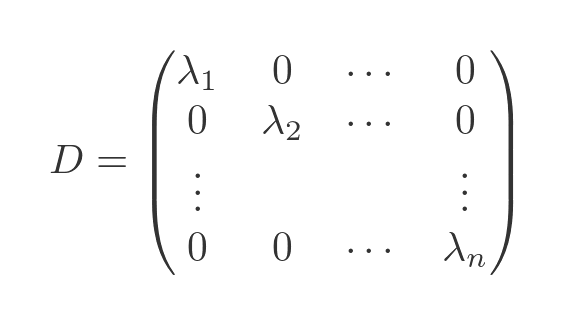
2. Construct \(D\), the diagonal matrix where eigenvalues appear along the diagonal.

\(D = \text{diag}(\lambda_1, \lambda_2, \dots, \lambda_n)\)

Example:

For eigenvectors \(v_1 = \begin{bmatrix} 1 \\ 0 \end{bmatrix}\), \(v_2 = \begin{bmatrix} 0 \\ 1 \end{bmatrix}\) and eigenvalues \(\lambda_1 = 1\), \(\lambda_2 = 5\):

\(S = \begin{bmatrix} 1 & 0 \\ 0 & 1 \end{bmatrix}, \; D = \begin{bmatrix} 1 & 0 \\ 0 & 5 \end{bmatrix}\)

\(H3: Optional: Compute \( S^{-1} \)\)

To complete the diagonalization formula:

\(S^{-1}AS = D\)

Compute \(S^{-1}\), the inverse of \(S\):

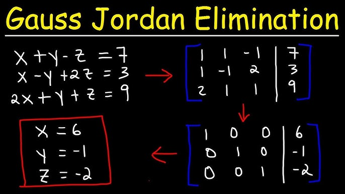
1. Use row reduction (Gauss-Jordan elimination) to compute \(S^{-1}\): Append \(I\) to \(S\), and transform \(S\) into \(I\), while \(I\) becomes \(S^{-1}\). 

2. Alternatively, for 2×2 matrices, use the formula:

\(S^{-1} = \frac{1}{\text{det}(S)} \begin{bmatrix} d & -b \\ -c & a \end{bmatrix}, \; \text{for } S = \begin{bmatrix} a & b \\ c & d \end{bmatrix}\)

Example:

If \(S = \begin{bmatrix} 1 & 2 \\ 3 & 4 \end{bmatrix}\), then:

\(\text{det}(S) = 1 \cdot 4 - 2 \cdot 3 = -2\)

\(S^{-1} = -\frac{1}{2} \begin{bmatrix} 4 & -2 \\ -3 & 1 \end{bmatrix}\)

Practical Tip: To verify correctness of \(S^{-1}\), check that multiplying \(S \cdot S^{-1} = I\).

Step 6 - Verify the Diagonalization

Finally, confirm the diagonalization by checking:

\(S^{-1}AS = D\)

Steps to verify:

1. Multiply \(S^{-1}\) and \(A\), then multiply the result with \(S\).

2. Confirm that the product reduces to \(D\).

Example:

For \(A = \begin{bmatrix} 4 & -1 \\ 2 & 1 \end{bmatrix}\):

If \(S = \begin{bmatrix} 1 & 2 \\ 2 & 1 \end{bmatrix}\), \(D = \begin{bmatrix} 3 & 0 \\ 0 & 2 \end{bmatrix}\):

1. Compute \(S^{-1}AS\).

2. Verify all diagonal entries of \(D\) match the corresponding eigenvalues.

Applications of Diagonalization

Simplifying Matrix Computations

One primary benefit of diagonalization is the ability to simplify matrix operations, particularly matrix powers. Suppose \(A\) is diagonalizable, then:

\(A^n = S D^n S^{-1}\)

Raising a diagonal matrix \(D\) to the \(n\)-th power is straightforward since:

\(D^n = \text{diag}(\lambda_1^n, \lambda_2^n, \dots, \lambda_n^n)\)

Example:

For \(A = \begin{bmatrix} 2 & 0 \\ 0 & 3 \end{bmatrix}\), \(D = A\):

\(A^5 = \begin{bmatrix} 2 & 0 \\ 0 & 3 \end{bmatrix}^5 = \begin{bmatrix} 2^5 & 0 \\ 0 & 3^5 \end{bmatrix} = \begin{bmatrix} 32 & 0 \\ 0 & 243 \end{bmatrix}\)

This characteristic is notably advantageous for examining sustained behavioral patterns in ecological populations or constructing simulations of mechanical systems.

Solving Systems of Linear Differential Equations

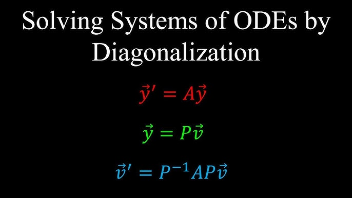
Diagonalization is a powerful tool for solving systems of linear differential equations. Systems expressed as \(\dot{x} = Ax\), where \(x\) is a vector and \(A\) is a coefficient matrix, can be simplified using diagonalization:

1. Suppose \(A = S D S^{-1}\). Write \(\dot{x} = S D S^{-1}x\).

2. Substitute \(y = S^{-1}x\): \(\dot{y} = D y\).

3. Solve the decoupled system \(\dot{y}_i = \lambda_i y_i\) for each \(y_i\).

4. Transform back: \(x = S y\).

In physics, diagonalization is used in quantum mechanics to decouple Schrödinger equations, enabling solutions for independent energy states.

Beyond Basics: Nontraditional Perspectives on Diagonalization

Non-Diagonalizable Matrices and "Jordan Normal Form"

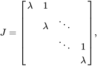
While diagonalization is highly useful, not all matrices can be diagonalized. For defective matrices—those that lack enough linearly independent eigenvectors—the concept of Jordan Normal Form (or Jordan Canonical Form) provides an alternative. Rather than generating a diagonal matrix, the transformation yields a block-diagonal arrangement in which individual blocks associate with eigenvalues yet can incorporate coupled entries termed Jordan blocks.

Example:

For a defective matrix \(A = \begin{bmatrix} 5 & 1 \\ 0 & 5 \end{bmatrix}\) with eigenvalue \(\lambda = 5\) of algebraic multiplicity 2 but geometric multiplicity 1, diagonalization is not possible. However, the Jordan Normal Form is:

\(J = \begin{bmatrix} 5 & 1 \\ 0 & 5 \end{bmatrix}\)

Jordan Form allows us to work with such matrices for applications requiring matrix powers or solving differential equations. Although slightly more complex than diagonalization, the Jordan Form ensures matrix analysis remains feasible even in challenging cases.

Connection to Machine Learning and Data Science

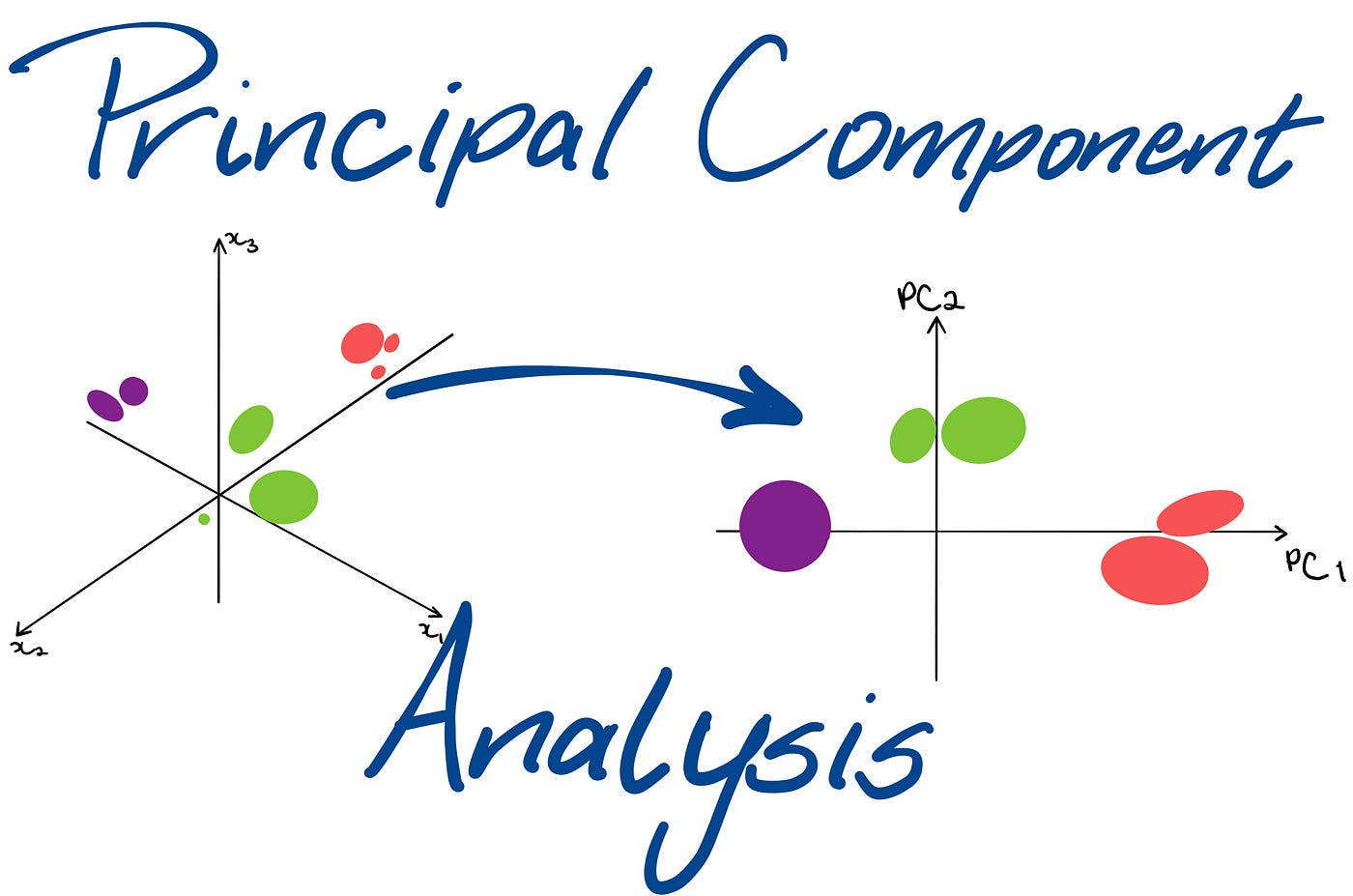
Diagonalization plays a crucial role in Principal Component Analysis (PCA), a dimensionality-reduction technique used to simplify datasets with many variables. In PCA:

1. The covariance matrix \(\Sigma\) of the data is computed.

2. The eigenvalues and eigenvectors of \(\Sigma\) are determined.

3. Eigenvectors define new "principal axes" (directions of maximum variance), and their corresponding eigenvalues indicate the level of variance captured.

Example: In image processing, diagonalization is used to compress high-dimensional images by projecting them onto the top-k principal components. This essentially reduces the storage requirements while preserving critical features. For instance, eigenvalue decomposition can simplify high-dimensional face recognition datasets, improving computational efficiency in machine learning.

FAQs and Common Pitfalls

Frequently Asked Questions

What happens if all eigenvalues are complex numbers?

Complex eigenvalues often emerge in real matrices for rotation or oscillatory transformations. Though such matrices cannot be diagonalized over real numbers, complex numbers allow their diagonalization instead.

Can all matrices be diagonalized?

No. To be diagonalized, a matrix must contain enough linearly independent eigenvectors which are linearly independent of each other and sufficient linear multiplicity for its algebraic multiplicity to outweigh geometric multiplicity; any defective matrix cannot be diagonalized due to geometric multiplicity being less than algebraic multiplicity.

Mistakes to Avoid During Diagonalization

- Mismatching eigenvectors and eigenvalues: Ensure each eigenvalue corresponds to its eigenvector in constructing matrices \(S\) and \(D\).

- Overlooking multiplicity checks: Always verify that the geometric multiplicity matches the algebraic multiplicity for all eigenvalues.

- Inverse computation errors: When computing \(S^{-1}\), numerical errors, particularly for ill-conditioned matrices, can lead to incorrect results. Double-check results to ensure consistent multiplication \(S \cdot S^{-1} = I\).

Conclusion

Diagonalization is a transformative process that simplifies matrix computations. The steps include:

1. Finding the characteristic polynomial and solving for eigenvalues.

2. Computing eigenvectors and verifying geometric and algebraic multiplicities.

3. Constructing the matrices \(S\) (eigenvectors) and \(D\) (eigenvalues on the diagonal).

Diagonalization enables complex operations like matrix powers or solving differential equations to be transformed into simpler and more computationally efficient tasks by diagonalization.

Matrix diagonalization is one of the cornerstones of linear algebra and finds applications across physics, engineering and machine learning. Through mastering this concept you unlock power to analyze datasets, solve dynamic systems and streamline computation. For advanced topics try Jordan Normal Form or numerical methods for diagonalizing large matrices like Python or MATLAB programming environments.

Reference:

https://math.stackexchange.com/questions/3060423/calculation-of-jordan-normal-form-to-determine-similarity

https://textbooks.math.gatech.edu/ila/characteristic-polynomial.html

https://builtin.com/data-science/step-step-explanation-principal-component-analysis