How to Find the Equation of a Line?

What Is a Linear Equation?

Definition and Components

Definition & Structure

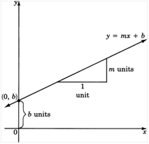
A linear equation is a mathematical representation of a straight-line relationship between two variables. It is usually expressed as y = mx + c.

m represents the slope, which is the measure of the line’s steepness or incline. A higher value of m indicates a steeper line.

C indicates the y-intercept, the point at which a line crosses over onto its respective y-axis and marks out where its starting position starts relative to y. Together m and c provide an easy to comprehend and highly applicable format that describes all aspects of straight lines geometry.

Applicability

Linear equations play an essential role in mathematical modeling, financial forecasting, engineering design, and social sciences - from budget modeling proportional to production quantities to tracking speed over time in physical systems - using linear equations provides a simple yet powerful means of characterizing their behaviors. For instance, expenses proportional to production quantities or speed over time in physical systems can all be represented using these simple yet effective mathematical expressions.

Rearranging Equations

Not all equations can be represented using the slope-intercept form (y=mx+c). Consider, for instance, equations such as 2y-4x=6, which must be modified in order to isolate y. In this instance:

2y−4x=6⟹y=2x+3.

Rearranging simplifies an equation's structure and makes its slope (m=2) and y-intercept (c=3) easy to identify while simplifying graphing and interpreting its relationship among variables.

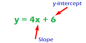
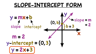
Slope-Intercept Form

Definition and Concept of Slope-Intercept Form

Basic Structure

Slope-intercept form (y=mx+c) is an established format for linear equations. The slope (m) defines how steeply or steeply a line rises or falls; for instance, an increase of one unit in x will cause an equal increase in y. For instance, when set as five this means for every 1-unit increase of x, five units increase will cause five increases of y to appear simultaneously.
The y-intercept (c) defines where a line crosses over to cross the y-axis and anchoring itself to its graph at x=0. Not only is this form visually intuitive but it allows quick calculations when provided slope and y-intercept values are provided.

Direct Application

When slope m and y-intercept c are known, creating a linear equation becomes a simple plug-and-play process. For example, if a car rental company charges a 50 base fee (c) and 0.20 per mile (m), the total cost equation is y=0.2x+50, where x represents miles driven.

Steps to Solve

Step 1

Identify the slope (m) and y-intercept (c). Often, these values are provided directly in the problem.

Step 2

Substitute the identified slope and intercept into y=mx+c.
For example, given m=−3 and c=6, the resulting equation is:

y=−3x+6.

Quick Validation Method

Test the equation by substituting a known point. For the example above (y=−3x+6), substitute x=2:

y=−3(2)+6=0.

When this matches up with the expected value, it means the equation has been correctly predicted and applied. This method provides an additional layer of confidence, particularly useful in exams or problem-solving scenarios where precision matters.

Point-Slope Form

Definition and Concept of Point-Slope Form

General Formula

The point-slope form of a linear equation is expressed as:

\(y−y_{1}​=m(x−x_{1}​)\),

where m represents the slope, and (\(x_{1} ​,y_{1}\)) denotes a point on the line.This form is ideal for situations where you are provided with the slope and at least one specific point but lack the y-intercept.

Steps to Solve

Step 1

Calculate or identify the slope (m). This might require using the formula for slope if not directly provided:

\(m= \frac{y_{2} -y_{1} }{x_{2} -x_{1}} ​​.\)

Step 2

Select a known point (\(x_{1}​,y_{1}​\)) from the problem’s context.

Step 3

Substitute the slope and point into the formula. For instance, using m=4 and point (1,3):

y−3=4(x−1).

Step 4

Simplify into slope-intercept form (y=mx+c), if necessary. Expanding on the above example:

y−3=4x−4⟹y=4x−1.

Validation with Geometry

Visually test an equation's accuracy by graphing its given point and plotting out its slope; for instance, plotting (1,3) along a gradient of 4 will create a line consistent with its equation y=4x-1; this two step approach reinforces both understanding and accuracy simultaneously.

Why Parallel and Perpendicular Lines Are Special

Properties of Parallel Lines

Definition and Key Feature

Parallel lines share the same slope (\(m_{1}​=m_{2}​\)) but have distinct y-intercepts. This means they never intersect and maintain a constant distance apart across the graph.

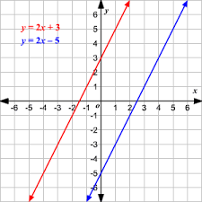
Steps to Solve Parallel Line Equations

Identify the slope (m) of the given line.

Use the same slope with the new point provided for the parallel line in the point-slope form.

For instance, if the line y=3x+2 is parallel to another line passing through (4,10):

y−10=3(x−4)⟹y=3x−2

Properties of Perpendicular Lines

Negative Reciprocal Relationship

If two lines are perpendicular, their slopes multiply to −1. For example, if one slope is m=2, the perpendicular slope is \(m=−\frac{1}{2}\).

Example Problem

Given line \(y=\frac{1}{3} ​x+2\), find the perpendicular line passing through (6,−1):

m=−3, so y+1=−3(x−6)⟹y=−3x+17.

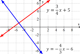
Understanding Through Symmetry

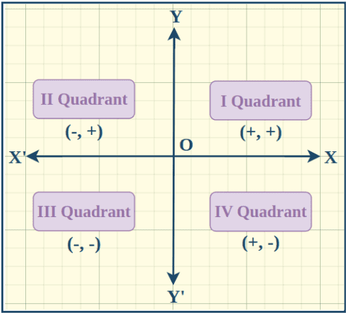
The concept of symmetry offers a clear way to understand perpendicular lines. Visualize the original line as a mirror axis on a graph, with the perpendicular line crossing it at a 90-degree angle—this provides an intuitive way to comprehend their relationship. Slopes of these lines that are negative reciprocals create an equilibrium when balanced symmetrically; for instance, if one line has an upward slope \(m_{1}=2\), another one would follow and feature an oppositely directed slope of \(m_{2} =-\frac{1}{2}\); this way we create a balanced design. When two lines meet on a graph, their intersection will form consistent right angles, which visually divide it into four equal quadrants. Plotting further highlights this symmetry: each rise and run of one line is mirror-imaged on its counterpart for added perpendicularity during slope calculations and spatial alignment purposes.

Real-World Applications

Practical Usage

Linear equations have long been utilized by businesses as an invaluable way of modeling quantitative relationships across industries. Businesses utilize them for forecasting demand, setting pricing strategies, and estimating profitability; one example is using revenue equations such as 40x+200 to forecast demand or estimate profitability from sales volume data. Linear equations also model transportation costs per mile to optimize fuel and labor use while improving pricing accuracy and decision-making accuracy in logistics companies or even online retailers that use distance or weight-based shipping calculations when shipping packages; all this illustrates how linear equations transform data into actionable insights and informed business strategies!

Planning and Optimization

Linear equations play a central role in resource planning and cost optimization across industries like manufacturing, supply chains, and project budgeting. Models like 50x+500 (where x is output, 50 is variable cost per unit, and 500 fixed costs are defined respectively) help determine cost-effective production levels while streamlining supply chains by optimizing transportation costs with delivery schedules to minimize expenses. Project managers employ linear equations for forecasting expenses by dissecting expenses such as hourly labor rates from fixed ones such as equipment rentals to create clear models - tools that enable businesses to simulate outcomes and maximize efficiencies while making informed financial decisions and business simulation outcomes as they plan and budget accordingly.

Using Graphs to Find Linear Equations

Graphs are an incredibly visual and intuitive way of analyzing relationships between variables. When working with linear equations, graphs provide an excellent means to derive key components such as slope and y-intercept directly. This section emphasizes both manual graph analysis for ideal data and computational methods for irregular or scattered data.

Identifying Slope and Intercept from a Graph

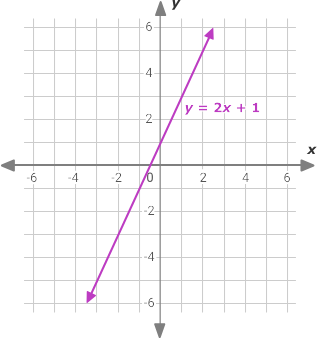
Extract Data

To determine the equation of a line from a graph:

1. Identify its equation from its graphed line: Mark at least two clearly identifiable points on its line that lie near grid intersections for easier calculation and less error; examples might include (1,3) and (4,9) as such points could work well as starting points.

2. Use these two points to calculate the slope (m), which is the ratio of the vertical change (\(\bigtriangleup y\)) to the horizontal change (\(\bigtriangleup x\)):

\(\frac{\bigtriangleup y }{\bigtriangleup x} =\frac{9-3}{4-1} =\frac{6}{3} =2\)

3. Observe where the line intersects the y-axis to determine the y-intercept (c). For example, let’s assume the graph crosses the y-axis at (0,1), making c=1.

Combine Components

Now, substitute these values into the slope-intercept form y=mx+c. The resulting equation is:

y=2x+1.

Dealing with Irregular Data

Trend Lines for Scattered Data

Real-world applications involve noisy data. A graph is typically messy, with points scattered rather than falling perfectly along a straight line. To derive meaningful linear relationships:

Approximating via Trend Lines : Draw a trend line which best matches the distribution of points, representing their average behavior as data and helping you estimate slope and intercept.

Computational Support : Utilize software such as Excel, Google Sheets or Python libraries to construct the best-fit line using linear regression. Such tools estimate slope (m) and intercept (c), by minimizing errors between actual points and predicted values.

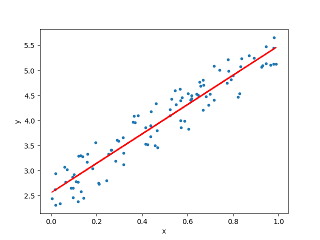
By providing strategies that address both ideal graph lines and irregular data points, this approach equips you to tackle various graph-derived linear equations.

Common Mistakes and How to Avoid Them

Mistakes in solving or interpreting linear equations are common but can be avoided with careful attention to detail and methodical problem-solving.

Confusion Between Slope and Intercept

Issue

A frequent error is confusing the slope (m) with the y-intercept (c). Many confuse the coefficient of x (m) as the intercept or vice versa. This happens because they fail to distinguish between the roles of these two elements:

Slope (m) describes the line's steepness and the rate of change.

Y-intercept (c) determines where the line intersects the y-axis at x=0.

Solution

Always link each term back to its geometric meaning on the graph as you work. Practicing graph-based visualizations can solidify these concepts.

Error in Signs Of Coordinate

Issue

Errors often occur when handling positive and negative coordinates, particularly if one dimension (e.g.,x or y) involves negative values. For instance, when performing calculations like \(\bigtriangleup y=y_{2}-y_{1}\)​, forgetting one y value's negative sign invalidates it entirely and renders your calculations invalid.

Solution

Double-check all coordinates before computing slope or intercept and explicitly write each sign during calculations.

Misjudging  \(\bigtriangleup x\) or \(\bigtriangleup y\)

Issue

Misinterpreting the graph’s scale can lead to errors in calculating the change in x (\(\bigtriangleup x\)) or y (\(\bigtriangleup y\)). For example, assuming a grid increment represents 1 instead of 0.5 could result in a slope error.

Solution

Carefully examine the graph’s axis labels and use precise measurements when determining rise over run.

Advanced Applications and Tools

Linear equations provide a gateway to even more advanced mathematical problem-solving. Leveraging technology and extending concepts beyond single-variable relationships allows for broader analysis and insights.

Multi-variable Linear Equations

While basic linear equations involve only two variables (x and y), many systems need multiple variables in order to accurately model complex situations, including:
Forecasting profits requires accounting for labor (\(x_{1}\)), material (\(x_{2}\)) and overhead costs (\(x_{3}\)) when forecasting profits; the result may look something like this:\(y=50x_{1} +40x_{2} ​+100x_{3} ​+500\). This approach helps businesses and researchers analyze multiple influencing factors simultaneously.

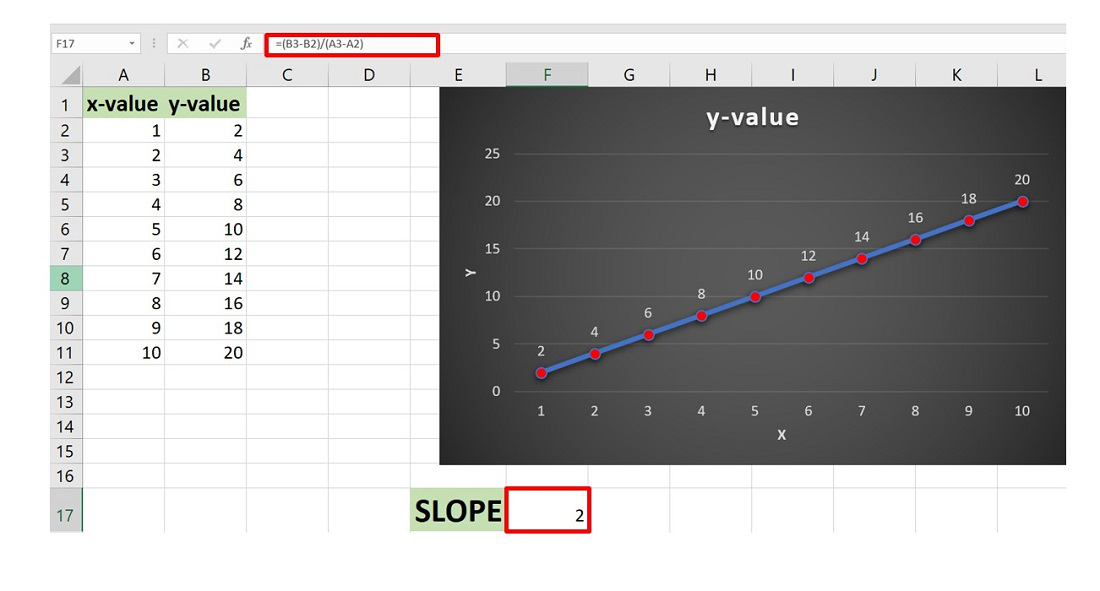
Leveraging Software for Calculations

Modern tools simplify linear regression, data analysis, and graph plotting. For example:

Excel or Google Sheets

Built-in functions like LINEST are used to derive slope and intercept values from data points.

Python with Matplotlib or NumPy

Plot data efficiently, calculate best-fit lines quickly, and visualize equations easily using Python script. A script can analyze hundreds of data points quickly for large datasets - ideal for fast yet accurate explorations of linear behaviors while eliminating manual errors.

Conclusion

Linear equations are practical tools that bridge mathematical theory and real-world applications. By mastering methods like slope-intercept form, point-slope form, and the two-point method, you can effectively solve a wide range of problems. These equations help model relationships, predict trends, and optimize decisions across industries, from science to business.

Understanding linear concepts, whether through graphing, working with parallel and perpendicular lines, or applying computational tools, provides valuable skills for both academic and professional growth. As you continue exploring, linear equations will serve as a reliable foundation for tackling more complex challenges and interpreting real-world data with precision.

Reference：

https://www.simplilearn.com/tutorials/excel-tutorial/data-analysis-excel

https://www.mdpi.com/2078-2489/11/4/193

https://www.statology.org/predictions-regression/