How to Find Rank of a Matrix?

Introduction to Matrix Rank

What is the Rank of a Matrix?

In linear algebra, rank is an essential concept that measures the dimension of vector space spanned by its rows or columns. More simply put, rank shows how much "information" or independent rows or columns a matrix holds. For example, consider a matrix \(A\) that has rows or columns that can be written as linear combinations of others. The rank reflects the number of truly essential, independent rows or columns.

Mathematically, the rank of a matrix may be defined as follows:

1. Maximum number of linearly independent rows (row rank).

2. The maximum number of linearly independent columns (column rank).

A key theorem in linear algebra states that row rank and column rank always sum to one; when taken together, they form what's known as matrix rank.

Example:

If matrix \(A = \begin{bmatrix} 1 & 2 & 3 \\ 4 & 5 & 6 \\ 7 & 8 & 9 \end{bmatrix}\), the row rank is determined by assessing how many rows are linearly independent, and similarly, the column rank is checked for linear independence among columns. We will explore how to calculate this in detail later.

Why is Rank Important in Linear Algebra?

The rank of a matrix plays a significant role in the theory of linear systems of equations, transformations, and its applications across various fields such as statistics, computer science, and engineering. Intuitively, a rank-deficient matrix (where not all rows or columns are independent) lacks "full information" or "full dimension," which can restrict its usage.

Here are a few reasons why rank is crucial:

1. Solving Linear Systems:

The rank determines if an equation system contains one unique solution or infinite solutions, depending upon whether there exists only one unique or infinite solution for them.

2. Dimensional Representation:Rank can provide insight into the actual dimension of row and column vector spaces - this knowledge is crucial in both theoretical and applied linear algebra.

3. Applications in Machine Learning and Data Science: For applications such as principal component analysis (PCA) and singular value decomposition (SVD), matrix rank plays an instrumental role in understanding and simplifying data sets.

4. Understanding Transformations: In geometry, matrices represent linear transformations of vector spaces. Their rank provides insight into whether they compress dimensions or preserve them during transformations.

Matrix rank can serve both theoretical and practical needs for understanding structured data and transformations.

Key Properties of Matrix Rank

Fundamental Properties of Matrix Rank

Understanding the properties of rank is essential before diving into the methods for calculating it. Here are some fundamental properties and their implications.

Equality of Row and Column Ranks

As mentioned earlier, the rank of a matrix is both the row rank and column rank and these two are always equal. This is a central result in linear algebra.

- Example: For \(A = \begin{bmatrix} 1 & 2 & 3 \\ 4 & 5 & 6 \end{bmatrix}\), the row rank and column rank are both 2.

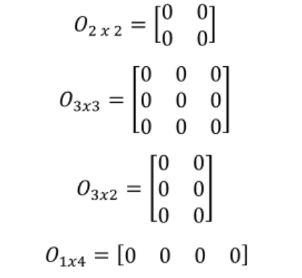
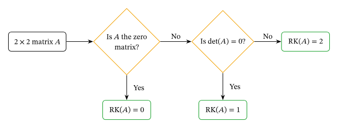
Rank of a Zero Matrix

A zero matrix contains no non-zero row or column vectors. Hence, the rank of a \(m \times n\) zero matrix is always 0.

\(A = \begin{bmatrix} 0 & 0 \\ 0 & 0 \end{bmatrix}\) has rank 0.

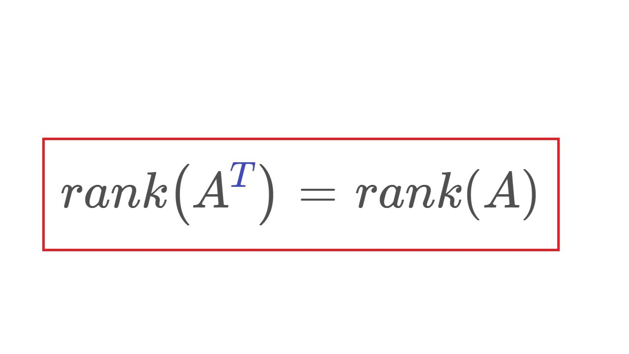
Rank and Matrix Transposition

The rank of a matrix remains unchanged under transposition. That is, \(\text{rank}(A) = \text{rank}(A^T)\).

Rank of a Product

If \(A\) is \(m \times n\) and \(B\) is \(n \times p\), \(\text{rank}(AB) \leq \min (\text{rank}(A), \text{rank}(B))\).

Addition of Matrices and Rank

In general, \(\text{rank}(A + B) \leq \text{rank}(A) + \text{rank}(B)\).

Rank of an Identity Matrix

The rank of an identity matrix \(I_n\) is \(n\), as all rows (or columns) of \(I_n\) are linearly independent.

Special Matrices and Their Ranks

Diagonal Matrix

For a diagonal matrix, the rank is simply the number of non-zero diagonal elements.

Upper or Lower Triangular Matrices

Similar to diagonal matrices, the rank equals the number of non-zero rows or columns.

Symmetric Matrix

Since symmetric matrices satisfy \(A = A^T\), their rank is invariant under transposition.

Singular vs. Non-Singular Matrices

A square matrix is singular if \(\text{det}(A) = 0\), which implies it is rank-deficient. Conversely, a non-singular matrix has a rank equal to its size.

Methods to Find the Rank of a Matrix

Method 1: Using the Minor Method

Step-by-Step Process

The minor method involves finding determinants of all possible square submatrices of a matrix. The largest size \(n\) for which a \(n \times n\) minor has a non-zero determinant gives the matrix rank.

1. Identify and extract all submatrices of the given matrix \(A\).

2. Compute the determinant for each square submatrix.

3. The rank is the size of the largest square submatrix whose determinant is non-zero.

Strengths and Limitations

- Strengths:  

The method is highly systematic and suitable for small matrices where submatrices can be computed manually.  

- Limitations:

It becomes computationally prohibitive as matrix size increases, given the exponential growth in the number of submatrices.

Example

Find the rank of \(A = \begin{bmatrix} 1 & 2 \\ 3 & 6 \end{bmatrix}\).  

Step 1: Determine all \(2 \times 2\) minors.  

\(\text{det}(A) = \text{det}\begin{bmatrix} 1 & 2 \\ 3 & 6 \end{bmatrix} = (1)(6)-(3)(2) = 0\)

Step 2: Check all \(1 \times 1\) minors. Non-zero determinants exist, so rank = 1.

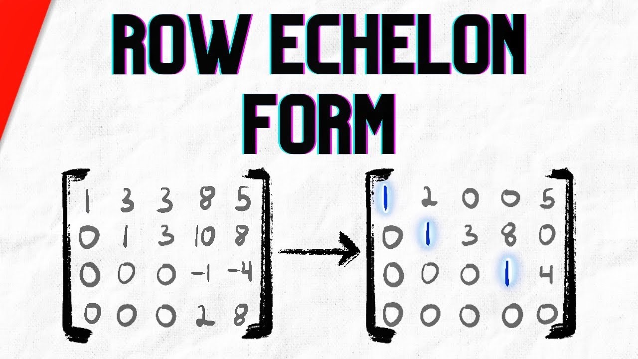
Method 2: Using Row Echelon Form

What is Echelon Form?

A matrix is said to be in row echelon form if:

1. All non-zero rows are above rows of all zeros.

2. The leading entry (also referred to as a pivot) of each non-zero row lies to the right of the leading entry in the row immediately above it.

3. All the elements in a column beneath a leading entry are zero.

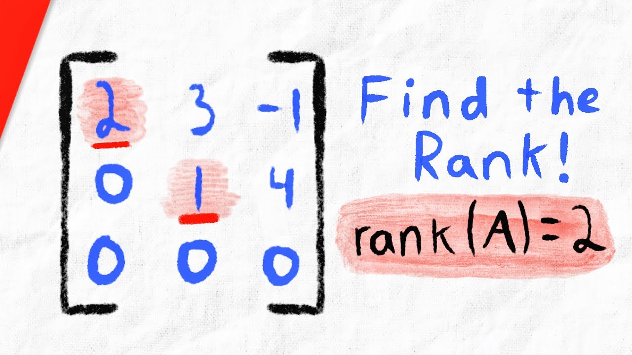
For example, this matrix is in row echelon form:\(\begin{bmatrix} 1 & 2 & 3 \\ 0 & 1 & 4 \\ 0 & 0 & 0 \end{bmatrix}\)

Step-by-Step Process

To calculate the rank of a matrix using REF:

1. Start with the given matrix \(A\): Write down the initial matrix.

2. Apply elementary row operations until the matrix is in row echelon form. Use techniques like row scaling, row swapping, and row addition/subtraction to zero out elements below the pivots.

3. Count non-zero rows: Once the matrix is in echelon form, the number of non-zero rows determines the rank of the matrix.

Column Transformations

Though row transformations are most frequently used, column transformations may also be beneficial (although less frequently). Instead of only considering row rank when applying column operations such as swapping columns or adding multiples of one column to another can help arrive at the matrix's column-echelon form, creating balance between row and column analyses by showing that their values match up perfectly - adding an equalizing element between analyses of rows vs columns.

 Example

Find the rank of \(A = \begin{bmatrix} 1 & 2 & 3 \\ 4 & 5 & 6 \\ 7 & 8 & 9 \end{bmatrix}\).

Step 1: Write the matrix.

\(A = \begin{bmatrix} 1 & 2 & 3 \\ 4 & 5 & 6 \\ 7 & 8 & 9 \end{bmatrix}\)

Step 2: Perform elementary row operations to get REF:

- Subtract 4*(Row 1) from Row 2:

\(\begin{bmatrix} 1 & 2 & 3 \\ 0 & -3 & -6 \\ 7 & 8 & 9 \end{bmatrix}\)

- Subtract 7*(Row 1) from Row 3:

\(\begin{bmatrix} 1 & 2 & 3 \\ 0 & -3 & -6 \\ 0 & -6 & -12 \end{bmatrix}\)

- Divide Row 2 by -3:

\(\begin{bmatrix} 1 & 2 & 3 \\ 0 & 1 & 2 \\ 0 & -6 & -12 \end{bmatrix}\)

- Add 6*(Row 2) to Row 3:

\(\begin{bmatrix} 1 & 2 & 3 \\ 0 & 1 & 2 \\ 0 & 0 & 0 \end{bmatrix}\)

Step 3: Count the non-zero rows:

The matrix in row echelon form has two non-zero rows. Hence, the rank of the matrix is 2.

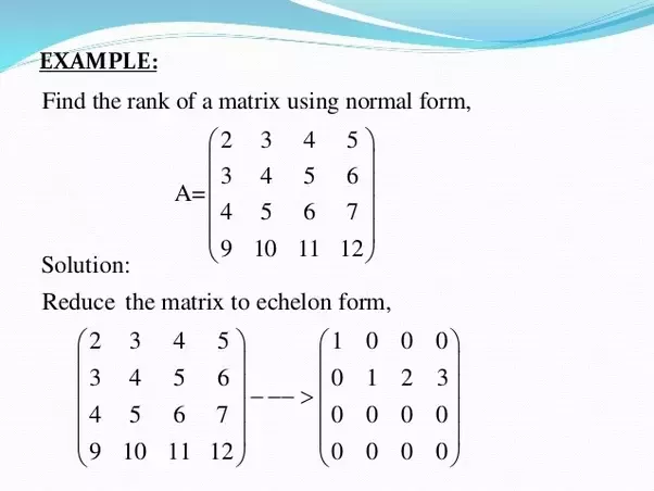
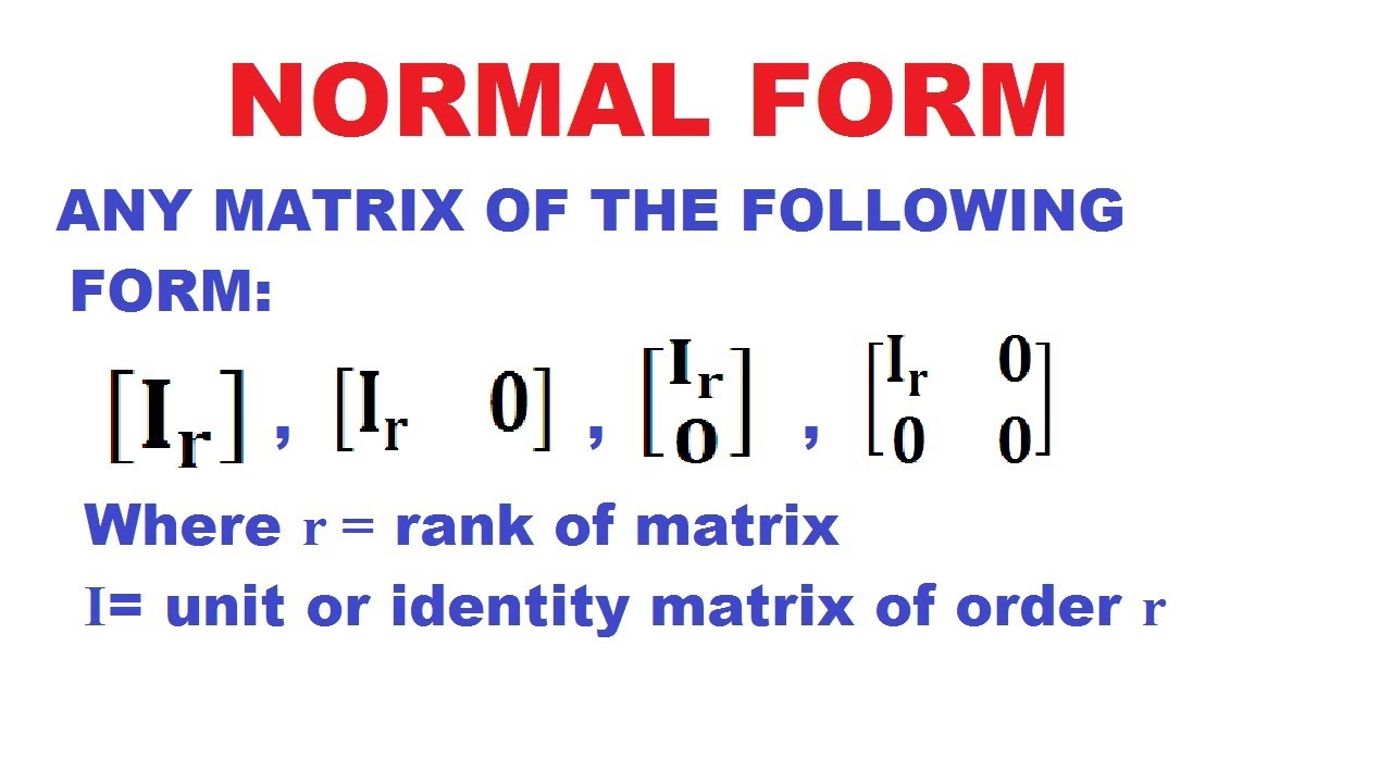
Method 3: Using Normal Form

What is Normal Form?

In linear algebra, the normal form of a matrix (or canonical form) refers to a simplified matrix that's equivalent to the original matrix but easier to analyze. One specific method is the "reduced row echelon form" (RREF), which refines the REF.

In RREF, every pivot is \(1\), and every column containing a pivot has zeros everywhere else. For example:

\(\begin{bmatrix} 1 & 0 & -5 \\ 0 & 1 & 4 \\ 0 & 0 & 0 \end{bmatrix}\)

Process

1. Begin with the original matrix.

2. Use elementary row operations, as in the REF method, to simplify the matrix.

3. Further refine pivot entries to ensure every pivot is \(1\) and all other entries in the pivot's column are zero.

4. The rank is still the number of non-zero rows.

Example

Consider \(A = \begin{bmatrix} 1 & 2 & 3 \\ 0 & 1 & 4 \\ 0 & 0 & 0 \end{bmatrix}\).

Already, the matrix is in REF.

To bring it to RREF:

- Divide Row 1 by \(1\):

\(\begin{bmatrix} 1 & 2 & 3 \\ 0 & 1 & 4 \\ 0 & 0 & 0 \end{bmatrix}\)

- Subtract \(2 \times (\text{Row 2})\) from Row 1:

\(\begin{bmatrix} 1 & 0 & -5 \\ 0 & 1 & 4 \\ 0 & 0 & 0 \end{bmatrix}\)

In RREF, there are two non-zero rows. The rank is 2.

Method 4: Singular Value Decomposition (SVD)

What is SVD?

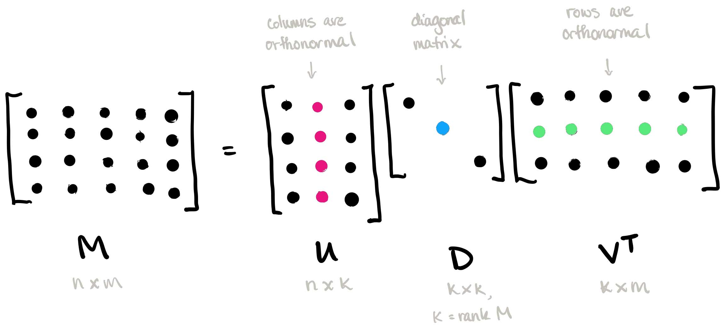
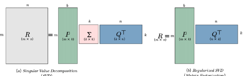
Singular Value Decomposition is an advanced linear algebra technique where a matrix \(A\) is factored into three matrices:

\(A = U \Sigma V^T\)

Here, \(U\) and \(V\) are orthogonal matrices, and \(\Sigma\) is a diagonal matrix containing the singular values of \(A\).

Application Scenarios

SVD is particularly useful in high-dimensional problems, such as:

1. Machine Learning and Statistics: Reducing the dimensionality of datasets.

2. Signal Processing: Reconstructing signals or images.

3. Numerical Analysis: Handling rank-deficient matrices.

Why Include SVD in Rank Calculation?

The rank of a matrix corresponds to the number of non-zero singular values in \(\Sigma\). This method offers high precision and robustness, even for noisy or high-dimensional matrices.

Example

If a matrix \(A = \begin{bmatrix} 1 & 1 \\ 0 & 0 \\ 1 & 1 \end{bmatrix}\), performing SVD yields singular values \(\sigma_1 = 2, \sigma_2 = 0\). The rank is **1**, as there’s only one non-zero singular value.

Comparing the Methods

Minor Method vs. Echelon Form

- Pros of Minor Method: Precise for small matrices; guarantees correct rank based on determinant calculations.

- Cons: Computational complexity for larger matrices.

- Pros of Echelon Form: Systematic and scalable to higher dimensions; easier to execute manually or programmatically.

- Cons: Requires mastery of row operations.

Echelon Form vs. Normal Form

- Echelon Form: Easier to compute and sufficient for most purposes.

- Normal Form (RREF): Refines results further, which is especially useful for verifying linear independence.

SVD and When to Use Advanced Techniques

SVD is overkill for simple matrices but unparalleled for large, complex systems where matrices are rank-deficient or near-singular. Use SVD for applications involving noise, approximations, or high precision.

Advanced Applications of Matrix Rank

Real-World Applications of Matrix Rank

Machine Learning

Principal Component Analysis (PCA), one of several techniques for dimensionality reduction in machine learning, relies heavily on covariance matrix rank when selecting features to be reduced based on rank; PCA can identify meaningful features based on rank to help effectively reduce dimensions while still preserving essential information. PCA allows practitioners to quickly find meaningful features of their dataset while still keeping essential details. Image recognition uses PCA extensively as it reduces computational complexity while simultaneously helping prevent overfitting by simplifying image data with a lower-rank matrix that captures its primary structure, making models faster and keeping accuracy intact.

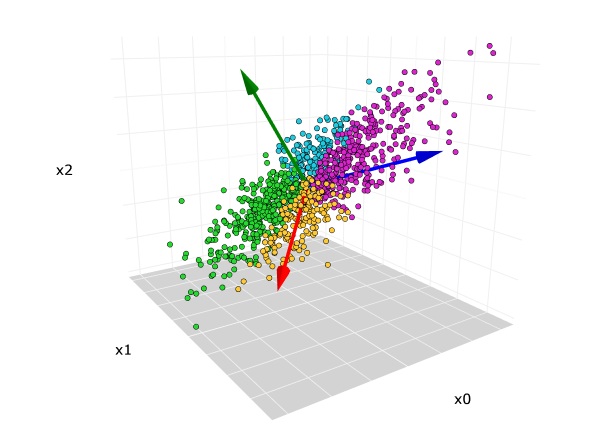
Image Compression

Image compression methods like JPEG depend on low-rank matrix approximations to efficiently reduce file sizes while maintaining visual quality. When applying Singular Value Decomposition (SVD) to an image matrix, only its most significant components (singular values) are kept. While less essential data such as "unimportant values" is lost. As a result of applying this low-rank approximation to create compressed files which almost look exactly the same but take significantly less storage space; making JPEG ideal for everyday digital photographs and videos!

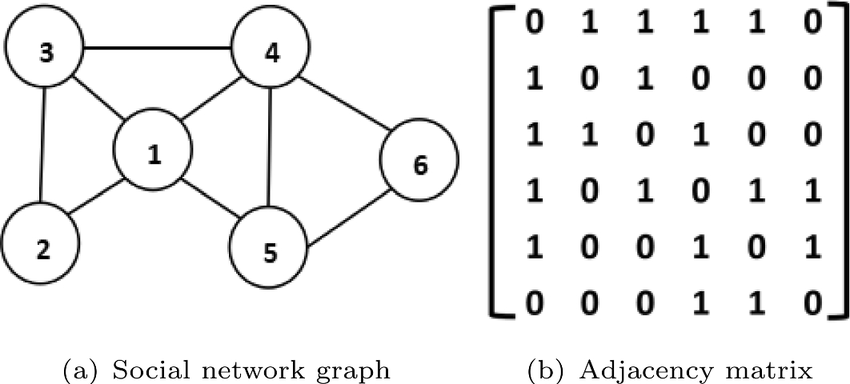
Network Analysis

Adjacency matrix ranks provide vital insight into the structure and connectivity of networks such as social media. They reveal independent communities or redundant connections within an overlapping social circle; low rank adjacency matrices might reveal clustered groups while full rank ones indicate more distributed and interconnected ones; such analysis helps identify key nodes or optimize network designs in areas like communication systems or transport grids.

Rank Sensitivity

Small perturbations in data (e.g., noise) can shift a matrix’s rank by introducing or destroying linear independence. Understanding this sensitivity improves methods for handling noisy datasets in disciplines like computational biology or signal processing.

FAQs on Finding the Rank of a Matrix

Popular Questions

Can a matrix’s rank exceed its smallest dimension?

No, the rank of a matrix cannot exceed its smallest dimension. For any matrix \(A\) of size \(m \times n\), its rank satisfies \(\text{rank}(A) \leq \min(m, n)\). This limitation arises from the definition of rank, as it represents the maximum number of linearly independent rows or columns in the matrix. In a geometric sense, the rank reflects the dimensionality of the space spanned by the matrix’s rows or columns, and this cannot exceed the actual number of rows (\(m\)) or columns (\(n\)) available.

For example, consider a \(2 \times 3\) matrix. While it has three columns, it can span at most a 2-dimensional subspace in a 3-dimensional space because there are only two rows to provide unique vectors. This principle ensures that the matrix rank respects the constraints of its physical dimensions.

Why are row and column ranks always equal?

The equality of row rank and column rank is an indispensable result in linear algebra, grounded in its relationship to matrix transformations, specifically the equality between row space dimensions and column space dimensions under any matrix transformation. Elementary row operations ensure this by upholding linear independence for rows and columns alike; this property lies at its heart by virtue of any matrix \(A\) being transformed into its row echelon form while still maintaining its rank; each non-zero row (row rank) corresponds directly with independent column count (column rank).

For instance, if a matrix has three linearly independent rows, the corresponding column space must also span three dimensions. This result guarantees that the dimensions of the two vector spaces—rows and columns—are inherently linked, leading to the key property: \(\text{row rank} = \text{column rank} = \text{rank}(A)\).

Why are rank-deficient matrices common in practice?

Real-world systems often include rank-deficient matrices due to data redundancy, measurement noise, or missing values that reduce the information content of the matrix; rank deficiency occurs when some rows or columns depend linearly upon one another, reducing the effective information content of the matrix - often occurring with datasets with related variables and repeated measurements which overlap information and lead to redundant rows/columns in an otherwise effective matrix structure.

Consider, for instance, a data matrix where age and birth year are both recorded - since these variables are mathematically intertwined, their inclusion creates redundancy, resulting in a rank deficiency in its matrix form. Sensor networks with multiple sensors measuring similar phenomena often experience this problem, with overlapped readings decreasing their rank value over time.

Rank deficiency can become even more prevalent when working with noisy or incomplete datasets, due to measurement errors introducing inconsistency or missing data sapping linear independence across rows or columns. Yet understanding and analyzing rank-deficient matrices remains vitally important when applying machine learning, signal processing or statistics techniques on noisy or incomplete datasets.

Conclusion

Understanding matrix rank connects theoretical concepts with practical applications in everyday life. From using traditional REF techniques or more modern SVD approaches to better comprehend its various properties - like finding solutions of linear systems to image compression applications - understanding matrix rank makes life simpler for both theoretical and real world applications of linear algebra.

Mastery of matrix rank can give you the tools needed to tackle problems across disciplines in math, science, and engineering, providing precision computational solutions and insight into data structures. So go ahead - calculate that rank! It will give you access to understanding how matrix computations operate!

Reference:

https://www.journalijar.com/article/17892/principal-component-analysis-as-a-ranking-tool---a-case-of-world-universities./

https://www.cs.cmu.edu/~venkatg/teaching/CStheory-infoage/book-chapter-4.pdf

https://www.quora.com/Why-does-the-column-rank-equal-the-row-rank-I-am-looking-for-intuition-based-answers-not-the-general-abstract-ones-available-in-textbooks