How to Multiply Matrices: A Comprehensive Guide

What is Matrix Multiplication?

Definition of Matrix Multiplication

A matrix is a structured, two-dimensional collection of numbers, symbols, or mathematical expressions systematically organized into rows and columns, forming a rectangular grid-like structure. Matrices serve as foundational constructs of mathematics in linear algebra as well as many branches thereof - with applications to various fields beyond just math, such as science and engineering - though many scientists consider matrices ideal storage solutions and effective means for performing sophisticated operations - matrix multiplication being one such operation that makes use of them very convenient.

Matrix multiplication is an elementary operation used in linear algebra that combines two matrices together and produces another matrix known as the product matrix, commonly used to represent linear transformations, solve systems of equations, and model real-world phenomena mathematically.

One essential feature of matrix multiplication is that it adheres to a strict compatibility rule: the first matrix's columns must correspond in number to the rows of the second matrix. In simpler terms, two matrices can only be multiplied if the "inner dimensions" match.

Example: If one matrix has dimensions m×n (m rows by n columns) while another one has dimensions n×p, multiplication should be valid and produce an output matrix with dimensions of m×p; otherwise, it would become undefined and the operation unknowable.

This rule derives from how matrix elements are combined: each entry in the product matrix represents an outcome from dot product between rows in one matrix and columns in another matrix, so dimension alignment becomes critical to successful matrix multiplication operations across different disciplines. Matrix multiplication not only captures numerical relationships but also geometric or algebraic connections - solidifying its position as an essential mathematical operation tool.

For example:

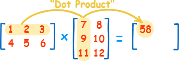
Matrix A is 2×3 :

\(\begin{bmatrix} 1 & 2 & 3\\ 4 & 5 &6\end{bmatrix}\)

Matrix B is 3×2 :

\(\begin{bmatrix} 7 &8 \\ 9 & 10\\ 11 &12\end{bmatrix}\)

The product of A and B will be a 2×2 matrix.

Applications and Importance

Matrix multiplication has long been considered an indispensable technique in computer science, physics, and economics for its ability to efficiently deal with complex data relationships. Artificial Intelligence/ML techniques also depend heavily on matrix multiplication, for example, when training neural networks, image recognition, text processing, or predictive modeling. Today's modern technologies often employ matrix operations directly. Tasks like facial recognition or recommendation systems also rely heavily on matrix operations; its presence is thus integral.

Matrix multiplication is essential across various fields, such as quantum mechanics and economics, where it models quantum states and transformations or aids in supply, demand, and resource optimization analysis. Furthermore, its versatility serves as the cornerstone of advancement across numerous scientific and technical fields alike.

Historical Background and Insights

Origins of Matrix Multiplication

Matrix multiplication dates back to Jacques Philippe Marie Binet of France's pioneering work on linear transformations and systems of linear equations in 1812. Binet pioneered matrix multiplication as an analytical tool. His contributions were motivated primarily by a need to develop efficient ways of representing and solving systems, which were central components of 19th-century mathematics and applied sciences. Binet initially focused his work on linear equations; his groundbreaking approach ultimately laid the foundations for linear algebra as a field. Over time, matrix multiplication became one of its hallmarks, providing deeper insights into vector spaces and transformations while impacting many different areas of mathematics and science.

Current Role in Mathematics

Matrix multiplication has quickly grown beyond its roots to become one of the most versatile and potency tools available to modern mathematics. Now, it is utilized across disciplines, from pure to applied sciences. Matrices are critical in quantum mechanics, representing operators that calculate probabilities and describe the behaviors of quantum systems. Matrices help model complex phenomena that would otherwise be difficult to formalize using more traditional means. Cryptography uses mathematical principles and codes to encrypt and transform data safely, providing a mathematical basis for protecting our digitally stored information in this digital era. Matrices provide an efficient means of solving optimization issues found in engineering, computer science, and economics by streamlining calculations to find efficient solutions to highly complex systems. Leading advancements in artificial intelligence and machine learning, large-scale matrix multiplications play an essential role in training neural networks, their effects being felt across fields as diverse as image recognition, natural language processing, and autonomous systems.

Matrix multiplication has many applications and stands as an indispensable building block, not only in theoretical mathematics but also for solving practical issues across a spectrum of scientific and technological fields.

Rules and Conditions for Matrix Multiplication

Core Rules of Matrix Multiplication

Compatibility Rule

For matrix multiplication to occur, the dimensions of the two matrices must adhere to the following:

If Matrix A has dimensions m×n and Matrix B has dimensions n×p, they are compatible.

The resulting matrix, Matrix C, will have dimensions m×p.

For example:

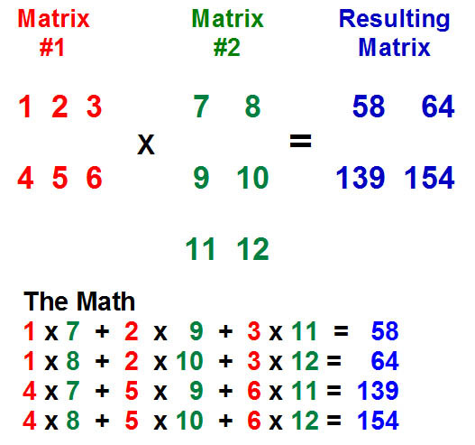
Matrix A (2×3):

\(\begin{bmatrix} 1 & 2 & 3\\ 4 & 5 &6\end{bmatrix}\)

Matrix B (3×2):

\(\begin{bmatrix} 7 &8 \\ 9 & 10\\ 11 &12\end{bmatrix}\)

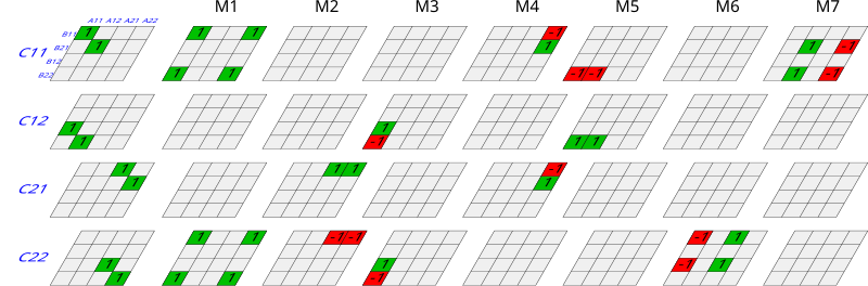
Matrix C (2×2) is computed as:

\(\begin{bmatrix} C11 & C12\\ C21 &C22\end{bmatrix}\)

Examples of Compatibility

A 3×2 matrix can be multiplied by a 2×4 matrix, yielding a 3×4 matrix.

A 4×3 matrix cannot be multiplied by another 4×3 matrix because the dimensions do not meet the compatibility requirement.

Commutativity and Special Cases

Non-Commutativity of Matrix Multiplication

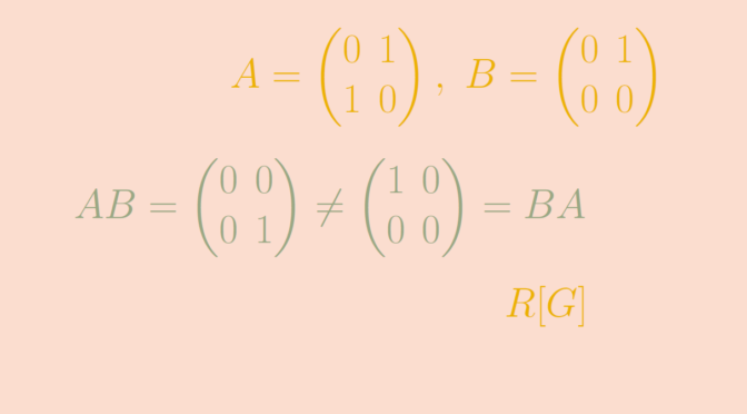
Matrix multiplication, unlike scalar multiplication, is not commutative. Generally, AB ≠ BA, even if both products are defined.

For example:

Let A and B be two 2×2 matrices:

\(A=\begin{bmatrix}1 &2\\ 3 &4\end{bmatrix}\)

\(B=\begin{bmatrix}5 &6\\ 7 &8\end{bmatrix}\)

Matrix AB:

\(\begin{bmatrix}1*5+2*7 &1*6+2*8\\ 3*5+4*7 &3*6+4*8\end{bmatrix}\)

\(=\begin{bmatrix}19 &22\\ 43 &50\end{bmatrix}\)

Matrix BA:

\(\begin{bmatrix}5*1+6*3 &5*2+6*4\\ 7*1+8*3 &7*2+8*4\end{bmatrix} =\begin{bmatrix}23 &34\\ 31 &46\end{bmatrix}\)

Clearly, AB ≠ BA.

Importance of Order in Real-World Applications

This property has real-life implications. For instance, in logistics, matrix multiplication order determines how supply chain data flows across geographical locations, impacting operational strategies and efficiency.

Identity and Zero Matrices

Identity Matrix

An identity matrix, denoted by I, is a square matrix with 1’s on its main diagonal and 0’s elsewhere. It preserves the values of other matrices during multiplication. For any matrix A:

A × I = A or I × A = A

For instance:

Identity Matrix (3×3):

\(\begin{bmatrix} 1&0 & 0\\ 0 &1 &0 \\0 & 0 &1\end{bmatrix}\)

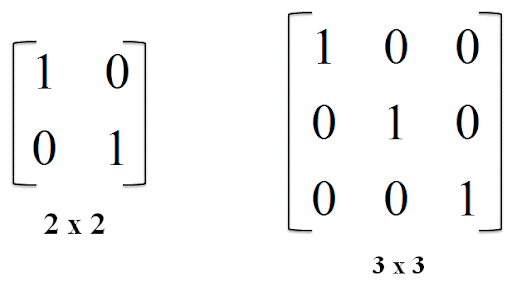
Zero Matrix

A zero matrix, denoted as O, consists solely of 0’s. Any matrix multiplied by the zero matrix yields another zero matrix:

A × O = O

Beyond Mathematics

These special matrices highlight the presence of dependencies or constraints within systems, reinforcing the principles of dependencies in fields such as physics or data models.

Step-by-Step Matrix Multiplication

Understanding Dot Product Operations

Row-by-Column Multiplier Formula

Calculating each element of the product matrix involves performing the dot product between a row of the first matrix and a column of the second:

Matrix A:

\(\begin{bmatrix} 1& 2\\ 3&4\end{bmatrix}\)

Matrix B:

\(\begin{bmatrix} 5& 6\\ 7&8\end{bmatrix}\)

Compute C[1,1]: (1×5) + (2×7) = 5 + 14 = 19

Compute C[1,2]: (1×6) + (2×8) = 6 + 16 = 22

Compute C[2,1]: (3×5) + (4×7) = 15 + 28 = 43

Compute C[2,2]: (3×6) + (4×8) = 18 + 32 = 50

Resulting Matrix C:

\(\begin{bmatrix} 19& 22\\ 43&50\end{bmatrix}\)

Common Errors

When performing this computation manually, the most common mistakes involve:

Misaligning rows and columns

Forgetting to ensure matrix dimensions are compatible

Manual Calculation Techniques

Visual Aids and Tools

To simplify manual calculations:

Use table grids to align elements row-by-column.

Highlight or circle corresponding values being multiplied.

Tricks to Tackle Large Matrices

For larger matrices like 4×4 or 5×5:

Break the matrix into smaller blocks.

Focus on calculating one quadrant or submatrix at a time.

Multiplication of Matrices with Different Dimensions

Matrix multiplication can take many forms depending on the dimensions of the matrices involved. While small matrices (e.g., 2×2) are easier to compute manually, larger matrices (e.g., 3×3 or high-dimensional ones) often require computational techniques. This section explores the step-by-step process for handling matrices of varying dimensions and demonstrates practical examples.

2×2 Matrix Multiplication

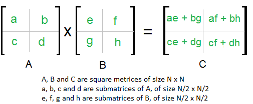
Calculating the product of two 2×2 matrices is a straightforward process. Given two matrices, A and B :

A =

\(\begin{bmatrix} a& b\\ c&d\end{bmatrix}\)

B =

\(\begin{bmatrix} e& f\\ g&h\end{bmatrix}\)

The product matrix C = AB will also have dimensions 2×2, and its elements are calculated as:

C =

\(\begin{bmatrix} ae+bg& af+bh\\ ce+dg&cf+dh\end{bmatrix}\)

Example

Suppose:

A = \(\begin{bmatrix} 1& 2\\ 3&4\end{bmatrix}\)

B = \(\begin{bmatrix} 5& 6\\ 7&8\end{bmatrix}\)

The resulting matrix C is computed as:

C[1,1] = (1*5) + (2*7) = 5 + 14 = 19  

C[1,2] = (1*6) + (2*8) = 6 + 16 = 22  

C[2,1] = (3*5) + (4*7) = 15 + 28 = 43  

C[2,2] = (3*6) + (4*8) = 18 + 32 = 50

Thus,

C = \(\begin{bmatrix} 19& 22\\ 43&50\end{bmatrix}\)

Applications of 2×2 Matrices

2×2 matrices are widely used in physics for simple system dynamics, such as spring-mass systems or 2D transformations (e.g., scaling, rotation).

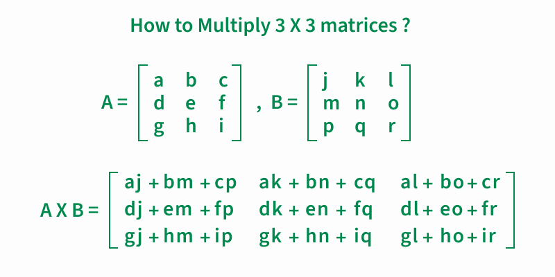
H3: 3×3 Matrix Multiplication

For 3×3 matrices, the principles remain the same, but the calculations increase in complexity due to the larger number of elements. Matrix A and B, both of dimensions 3×3, are given by:

A = \(\begin{bmatrix} a & b &c \\ d & e &f \\ g & h &i\end{bmatrix}\)

B = \(\begin{bmatrix} j & k &l \\ m& n & o \\ p & q & r\end{bmatrix}\)

The resulting matrix C = AB is computed by taking the dot product of each row of A with each column of B. Each element of C[i, j] is calculated as:

C[i, j] = A[i,1] × B[1,j] + A[i,2] × B[2,j] + A[i,3] × B[3,j]

Example

Given:

A = \(\begin{bmatrix} 1 & 2 & 3 \\ 4 & 5 & 6 \\ 7 & 8 & 9\end{bmatrix}\)

B = \(\begin{bmatrix} 10 & 11 & 12 \\ 13 & 14 & 15 \\ 16 & 17 & 18\end{bmatrix}\)

Calculating the first element C[1,1] :

C[1,1] = (1*10) + (2*13) + (3*16) = 10 + 26 + 48 = 84

Similarly, compute the rest to get:

\(\begin{bmatrix} 84 & 90 & 96 \\ 201 & 216 & 231 \\ 318 & 342 & 366\end{bmatrix}\)

Applications of 3×3 Matrices

3×3 matrices are frequently used in engineering (e.g., stiffness matrices in truss analysis).

In 3D computer graphics, they represent transformations like rotations and scaling in space.

High-Dimensional Matrix Multiplication

Multiplication becomes computationally expensive for larger matrix dimensions such as 4x4, 100x100, or beyond; its number of operations increases asymptotically with dimension; typical operations require O(n³) operations if done naively; thus, most high-dimensional matrices must be handled using advanced algorithms or software such as Python's NumPy library, MATLAB or TensorFlow designed for machine learning purposes.

Challenges of High-Dimensional Matrices

Memory Usage: Large matrices require substantial memory, especially when implemented on hardware like GPUs.

Computational Time: More dimensions exponentially increase computational time unless optimized algorithms like Strassen’s algorithm are used.

Example of Simplified Large-Scale Multiplication

Let A be a 100×50 matrix and B be a 50×100 matrix. Since each of the 100 rows in A must be multiplied by all columns of B, a total of 100×100 = 10,000 dot products are required.

Key Takeaways

Start with smaller dimensional matrices to build intuition for the multiplication rules.

Software tools are essential for handling large-scale operations in real-world applications like machine learning or quantum mechanics.

Properties of Matrix Multiplication

Matrix multiplication has several important mathematical properties that dictate how it behaves in different scenarios. These include the associative , distributive , and transpose properties . Further, determinants and special cases like diagonal and identity matrices lead to unique outcomes in multiplication.

Associativity of Matrix Multiplication

Matrix multiplication satisfies the associative property. For matrices A, B, and C, provided they are compatible for multiplication:

(AB)C = A(BC)

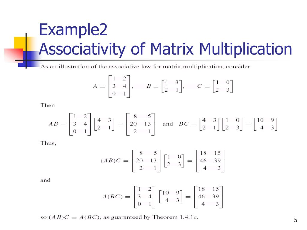
Example

Let:

A = \(\begin{bmatrix} 1 & 2\\ 3 & 4\end{bmatrix}\)

B = \(\begin{bmatrix} 5 & 6\\ 7 & 8\end{bmatrix}\)

C =\(\begin{bmatrix} 9 & 10\\ 11 & 12\end{bmatrix}\)

First, compute (AB)C : \(\begin{bmatrix} 19 & 22\\ 43 & 50\end{bmatrix}\)

Then, multiply by C:

[(AB)C] =  \(\begin{bmatrix} 19*9 + 22*11 & 19*10 + 22*12\\ 43*9 + 50*11 & 43*10 + 50*12\end{bmatrix}\)

Resulting in: \(\begin{bmatrix} 437 & 494\\ 1013 & 1146\end{bmatrix}\)

Now, compute A(BC) :

BC =  \(\begin{bmatrix} 152 & 168\\ 208 & 230\end{bmatrix}\)

Then, multiply A by this result:

A(BC) =\(\begin{bmatrix} 437 & 494\\ 1013 & 1146\end{bmatrix}\)

The final result confirms associativity.

Distributivity of Matrix Multiplication

Matrix multiplication also satisfies the distributive property:

A(B + C) = AB + AC

Example

Let:

A = [1 2]  

B = [3 4]  

C = [5 6]

Compute AB + AC and compare it to A(B+C). Both approaches yield the same result.

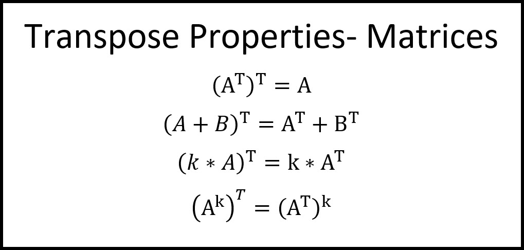
Transpose Property

For matrices A and B :

(AB)^T = B^T A^T

This property is critical in geometry and computer vision for rotating or scaling data.

Real-Life Applications of Matrix Multiplication

Matrix multiplication plays a vital role across various domains, powering innovations and solving complex problems in fields like machine learning, computer graphics, and physics. Far from being a mathematical abstraction, it is foundational to numerous real-world applications and technologies.

Machine Learning and Artificial Intelligence

Matrix multiplication lies at the core of machine learning and artificial intelligence systems, helping systems learn, predict, and recognize patterns. One key function for matrix multiplication lies within neural networks - an indispensable element in many AI programs that range from image recognition to natural language processing.

Neural networks rely on weight matrices that define relationships among neurons. When an input matrix (for instance pixel values or text embeddings) passes through, each layer multiplies it with weight matrices multiplicand create transformed outputs containing features extracted such as edges in images or semantic meaning in sentences for tasks like classification, translation or image recognition.

Deep learning models involve millions of matrix multiplication operations during training. These calculations enable the network to adjust and refine its weights through techniques like backpropagation for maximum accuracy and functionality. Matrix multiplication also forms an essential foundation of recommendation systems; techniques such as collaborative filtering or matrix factorization are used to predict user preferences via these methods; platforms like Amazon or Netflix depend heavily on such prediction capabilities to deliver tailored experiences to billions of customers worldwide.

GPUs and TPUs, specifically tailored for large-scale matrix calculations, have revolutionized AI applications like autonomous vehicles, virtual assistants, and real-time fraud detection by making AI much more accessible and efficient.

Computer Graphics

Matrix multiplication is at the core of computer graphics, enabling the manipulation and rendering of objects across 2D and 3D spaces. Matrix multiplication also supports essential transformations like scaling, rotation and translation that enable computer artists to produce realistic visuals in animated films, video games and simulations.

Imagine playing a video game: Every object in its world is represented as a matrix of coordinates, so when characters move, or the camera shifts, matrix multiplication recalculates these coordinates to reflect their new positions, ensuring seamless animation. A rotation matrix may alter an object's orientation while a translation matrix shifts its location within scenes; by chaining multiple transformations together through successive matrix multiplications, objects can be moved and sized up/down dynamically as needed.

Matrix multiplication plays an integral part in 3D environments, particularly processes like perspective projection. Perspective projection involves mapping 3D objects onto a 2D screen in order to simulate depth and realism - used extensively by virtual reality (VR) and augmented reality (AR) systems to adjust scenes according to user movements - real-time adjustments powered by matrix multiplication enable users to interact naturally within an artificially created world.

Computer-aided design (CAD) software leverages matrix multiplication to allow architects and designers to manipulate object geometries more precisely; without this mathematical foundation, immersive systems, lifelike simulations, and cinematic visuals in games or films wouldn't be possible.

Physics and Engineering

Physics and engineering use matrix multiplication extensively to model systems, solve equations and optimize designs. Many physical phenomena, from classical mechanics to quantum mechanics, are expressed mathematically through matrices.

In structural engineering, finite element analysis (FEA) involves dividing a structure into small components (finite elements) and representing their behavior—stress, strain, and deformation—using matrices. By multiplying and combining these matrices, engineers can predict how buildings, bridges, or vehicles respond to forces like loads or vibrations. This process ensures the safety and efficiency of designs ranging from skyscrapers to aircraft.

Matrix operations have long been used in physics to solve coupled systems of equations relating to orbital mechanics or particle interactions, representing orbital mechanics as orbital mechanics or interactions as interactions. Quantum mechanics particularly relies upon this mathematical foundation for representing states and operators using vectors and matrices - wave function transformations being one example modeled using multiplication between these matrices, while quantum computing also uses matrix multiplication techniques in order to describe quantum gates or simulate qubit manipulations.

Matrix multiplication also facilitates analysis of electrical circuits where components like resistances or voltages form interlinked networks, using Kirchhoff's circuit laws expressed as matrix multiplication to arrive at systematic solutions to complex electrical systems. Robotics and control systems likewise use matrix multiplication as an effective way to pinpoint precise movement paths for robotic arms or autonomous vehicles.

Matrix multiplication plays an essential role in connecting mathematical theory to practical engineering and scientific applications, from simulating physical dynamics to optimizing structural designs or processing energy systems.

Matrix multiplication has emerged as an indispensable component in shaping advances across machine learning, computer graphics and physics. From powering AI systems to rendering realistic visuals and solving scientific challenges - matrix multiplication's applications demonstrate its profound effect in shaping technologies while solving real world issues.

Challenges in Matrix Multiplication

Matrix multiplication, a fundamental operation in computational mathematics, faces several challenges due to its inherent computational and numerical complexity.

Numerical Errors

Matrix multiplication relies heavily on floating-point arithmetic, which is inherently prone to rounding errors due to the finite precision of computer representations. When multiplying large matrices or handling high-dimensional data, these small errors can accumulate, potentially leading to significant inaccuracies in the final result. This problem becomes more pronounced in iterative processes or applications like machine learning and scientific simulations, where matrices are multiplied repeatedly.

Computational Complexity

The brute-force method for matrix multiplication has an O(n³) time complexity - meaning its running time increases cubically as the matrix size grows larger. As datasets expand across fields such as artificial intelligence, big data analytics and scientific computing this becomes computationally expensive and time consuming - potentially becoming time and cost prohibitive when dealing with operations on very large matrices.

Optimized Solutions

Strassen’s Algorithm

Strassen's algorithm optimizes traditional matrix multiplication by reducing the number of multiplications involved. While it doesn't eliminate the cubic growth entirely, it lowers the complexity to approximately O(n².81), making it faster for sufficiently large matrices. However, the algorithm introduces additional overhead, such as complex data partitioning and increased memory usage, which can affect its real-world performance.

Parallel Processing

Parallel processing uses multicore CPUs or GPUs to distribute matrix multiplication across several processors or cores and accelerate it, speeding up computation significantly. Large-scale frameworks like CUDA for GPUs or distributed computing systems like Apache Spark may be utilized to speed up these operations significantly, though this approach reduces computation times significantly while creating challenges related to data synchronization and communication overhead between processors.

Conclusion and Future Perspectives

Matrix multiplication is more than a mathematical operation: it serves as a powerful tool that models, computes, and solves multidimensional, multivariate issues surrounding us every day. From designing transportation systems to teaching artificial intelligence how to predict outcomes accurately, correctly multiplying matrices enables us to systematically consider all elements within complex systems that make up life around us.

By way of this article, we have explored how matrix multiplication works and when and how it should be employed across disciplines. In particular, we identified rules concerning compatibility of dimensions associativity as well as challenges such as computational efficiency and precision errors that arise with this methodology.

Forward-thinking only stands to increase its significance; matrix multiplication serves as the cornerstone of cutting-edge fields such as quantum computing, where transformations of quantum states depend upon matrix multiplication; AI uses encoded weights within neural networks to power chatbots and image recognition services, among many other things;

Matrix multiplication holds great promise in novel fields like personalized medicine and environmental simulation, where large datasets require robust yet scalable computations to analyze them effectively. Mastering this mathematical operation not only facilitates careers within STEM disciplines but can be the solution to some of today's toughest problems.

Matrix multiplication serves as your guide in navigating interdependent relationships, whether they are subway routes, AI algorithms, dynamic systems in physics, or scaling dynamic systems. As we continue exploring innovation within computation and applications, this powerful operation will remain at the core of progress.

Reference:

https://medium.com/analytics-vidhya/linear-algebra-how-uses-in-artificial-intelligence-2e1e001c65

https://www.reddit.com/r/QuantumComputing/comments/1e0x1ad/can_quantum_computers_do_matrix_multiplications/

https://mathoverflow.net/questions/101531/how-fast-can-we-really-multiply-matrices