How to Solve Quadratic Equations?

Understanding Quadratic Equations

Definition and Standard Form (80 Words)

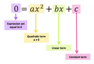
A quadratic equation is any equation that fits the standard form:

\(ax^{2} +bx+c=0\)

Where:

a, b, and c are constants.

a ≠ 0 (if a = 0, the equation reduces to a linear one).

A seemingly straightforward mathematical structure opens doors to many fascinating explorations in both mathematics and reality. Equation roots may take the form of real or complex numbers depending on how it's implemented into reality.

Breaking Down the Components

To better understand quadratic equations, let's break down their components:

ax²: The coefficient a determines the parabola's curvature or "width." Larger values of |a | create steeper parabolas, while smaller values flatten the curve.

bx: The linear coefficient impacts the parabola's symmetry and horizontal shift, altering where the vertex (turning point) lies.

c: Constant terms represent points where two lines intersect (x = 0).

They play an essential part in shaping and positioning parabolas and providing students with additional geometry-related problem-solving approaches to complement algebraic ones.

Types of Quadratic Equations

Quadratic equations come in various forms:

Complete Quadratics

Equations containing all terms (\(ax^{2}\) , bx , and c ), like:

\(2x^{2}+3x−5=0\)

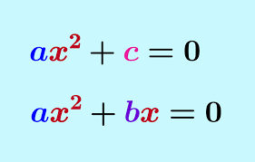
Incomplete Quadratics

Equations with missing terms, such as:

Only constant and square term remaining: \(x^{2}-16=0\)

Missing constant term: \(x^{2}+6x=0\)

Special Forms

These include variations like:

Factorable expressions: (x+3)(x−4)=0

Expanded forms requiring simplification, e.g., 3x(x−2)=6

Simplifying incomplete quadratic equations may accelerate the solving process for these cases.

Factoring to Solve Quadratic Equations

Step-by-Step Guide to Factoring

Factoring is one of the simplest and most intuitive methods to solve quadratic equations. Follow these steps:

Rearrange the Equation: Ensure the equation is in standard form:

\(ax^{2}+bx+c=0\)

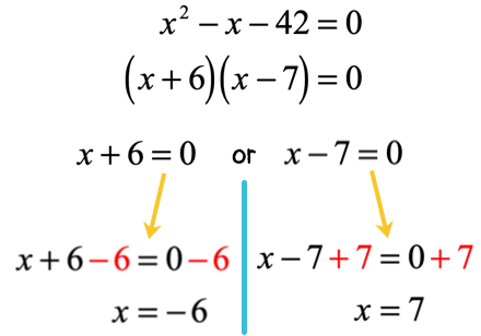
Identify Factors: Break the quadratic expression into a product of two binomials:

(px+q)(rx+s)=0

Set Each Factor to Zero: Solve for x by setting each binomial separately to zero:

px+q=0 and rx+s=0

Recognizing Factorable Quadratics

Not all quadratic equations are easily factorable. However, many exhibit recognizable patterns:

Perfect Square Trinomials: E.g., \(x^{2}+6x+9=(x+3)^{2}\).

Simple Integer Roots: Coefficients that provide straightforward factorization, like \(x^{2}+7x+10=(x+5)(x+2)\).

Original Insight: Identifying these patterns early can save time and effort during the problem-solving process.

Limitations of the Factoring Method

Although factoring is a powerful tool, it has limitations:

It only works when the quadratic is factorable with rational roots.

Complex or irrational roots require alternative methods, such as the quadratic formula or numerical techniques.

Using Graphical Approaches with Factoring

Another way to leverage factoring involves understanding its graphical implications. A factored quadratic equation corresponds to a parabola intersecting the x-axis at its roots. For example:

(x−2)(x+3)=0

On a graph, this would intersect at x=2 and x=−3.

Visualizing intersections allows students to hone their factoring abilities while building intuition about symmetry and root placement.

Solving by the Quadratic Formula

Introduction and Derivation of the Quadratic Formula

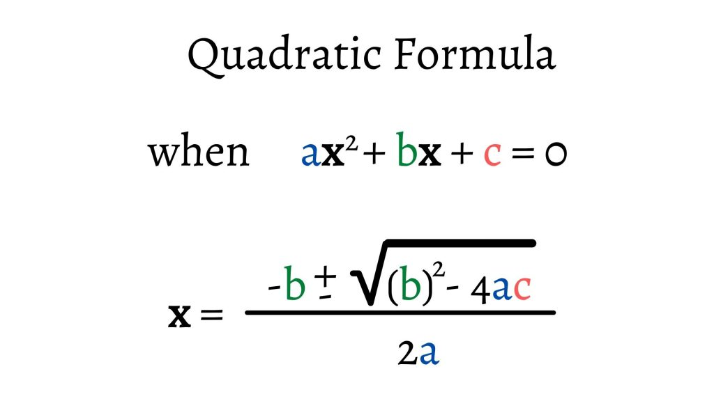
The quadratic formula is a comprehensive approach to solving any quadratic equation:

\(x=\frac{-b\pm\sqrt{b^{2}-4ac } }{2a}\)

It is derived by completing the square for the general quadratic equation:

\(ax^{2}+bx+c=0\)

Divide through by a to simplify.

Rearrange and complete the square by adding \((\frac{b}{2a} )^{2}\).

Solve for x, arriving at the quadratic formula.

Contrasting with factoring, this approach provides solutions for any quadratic equation with complex roots or non-rational roots, making it invaluable in more difficult equations.

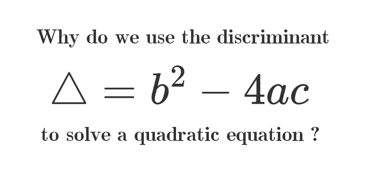
Role of the Discriminant (Δ)

The discriminant, \(Δ=b^{2}−4ac\), plays a crucial role within the quadratic formula, as it dictates the nature and quantity of roots:

Δ>0: Two distinct real roots.

Δ=0: One repeated (real) root.

Δ<0: Two complex roots.

For example, consider \(x^{2}−4x+4=0\). Here, Δ=0, indicating one repeated root, x=2.

By evaluating Δ early, students gain insight into the behavior of the equation and can plan their solving strategy accordingly.

Practical Application Steps

Solving a quadratic using the formula involves:

Identify coefficients: a, b, c.

Substitute into the formula:\(x=\frac{-b\pm\sqrt{b^{2}-4ac } }{2a}\)

Simplify results step-by-step.

For example, with \(2x^{2}+3x−2=0\):

a=2,b=3,c=−2.

\(Δ=3^{2}−4(2)(−2)=9+16=25\).

Roots: \(x=\frac{-3\pm5 }{4}\) ​, yielding x=0.5 and x=−2.

Solving by Completing the Square

What Is Completing the Square?

The method of completing the square involves rewriting a quadratic equation into the form of a perfect square trinomial. This technique allows us to express the quadratic equation in the following standard form:

\((x−h)^{2}=k\)

Here, h and k relate to the vertex of the parabola, offering valuable geometrical insights. Completing the square is particularly useful in situations where factoring is not possible, when deriving the quadratic formula, or in optimization problems.

For example, solving a quadratic equation like \(x^{2}+6x+5=0\) using this method reveals the connections between algebraic manipulations and parabolic transformations.

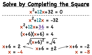
Step-by-Step Example

Step 1: Make the Coefficient of \(x_{2}\)  Equal to 1

If \(a\ne 1\) in the standard equation \(ax^{2} +bx+c=0\), divide the entire equation through by a to normalize the coefficient of \(x^{2}\).

For example: Solve \(2x^{2} +8x−10=0\). Divide by 2:

\(x^{2} +4x−5=0\)

Step 2: Add and Subtract Half the Linear Coefficient Squared

Add and subtract \((\frac{b}{2} ​)^{2}\), the square of half the linear coefficient, to create a perfect square trinomial on the left-hand side.

\(x^{2}+4x+(\frac{4}{2} )^{2}−(\frac{4}{2} )^{2}−5=0\)

Simplify:

\((x+2)^{2}−4−5=0\)

\((x+2)^{2}=9\)

Step 3: Solve Using the Square Root Property

Take the square root of both sides:

\(x+2=\pm \sqrt{9}\)

x+2=3 or x+2=−3

Solve for x:

x=1 or x=−5

Application of Completing the Square

Completing the square is closely tied to real-world problems such as maximizing profits in business, finding the maximum or minimum values in physics, and modeling geometric properties.

Understanding this method not only aids in solving equations but also builds insights into optimization problems, making it versatile across disciplines.

Graphical Method for Solving Quadratics

Basics of Graphing Quadratics

Graphical methods leverage the visual representation of quadratic equations as parabolas to identify their solutions. Recall that the general form of a quadratic equation, \(y=ax^{2}+bx+c\), produces a parabola when graphed.

Key Features of the Parabola:

Vertex: The vertex is the maximum or minimum point of a parabola, depending on whether it opens upwards (a>0) or downwards (a<0).

Axis of Symmetry: A vertical line that passes through the vertex, given by \(x=-\frac{b}{2a}\) ​.

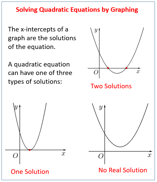
Roots (Solutions): The x-intercepts where y=0.

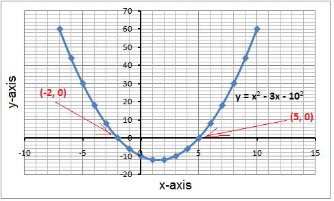
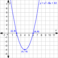
Finding Solutions Using Graphs

To solve a quadratic equation graphically, plot the parabola corresponding to \(y=ax^{2}+bx+c\). The x-coordinates of the points where the parabola intersects the x-axis represent the roots of the equation.

Case 1: Two Real Roots

In case one, where two distinct points on a parabola cross with two distinct x-axes at two distinct times, then this quadratic has two real solutions (real roots).

Case 2: One Repeated Root

When touching at only one vertex point, there will only ever be one repeated solution (Δ=0).

Case 3: No Real Roots

Unless the parabola intersects the x-axis in any way, there are no real solutions ((Δ<0; these solutions must be complex).

For example, the equation \(x^{2}−4x+3=0\) generates a parabola intersecting the x-axis at x=1 and x=3, corresponding to the roots.

Graphing with Modern Tools

Modern tools like Desmos, graphing calculators, and Python libraries simplify the process of visualizing quadratic functions. These tools provide precise visual representations, making it easier to analyze challenging equations or approximate roots when algebraic methods prove difficult.

Identifying the Most Efficient Method to Solve Quadratic Equations

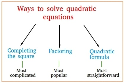
Overview of Solving Methods

Different quadratic-solving methods suit various scenarios:

Factoring can quickly solve simple equations with small coefficients, while the quadratic formula and completing the square are generally applicable solutions. For transformations or vertex issues, however, completion is the optimal approach.

Graphical methods excel at offering visualization and approximate solutions.

Decision-Making Framework

Selecting the best solving method depends on the equation's complexity and your goals:

Step 1: Start with Factoring

If the equation is simple and has rational roots, factoring is the fastest choice.

Step 2: Check the Discriminant Δ

Use the discriminant to decide:

If Δ>0, there are two real roots—consider factoring or the quadratic formula.

If Δ=0, one solution exists, suggesting completing the square or the quadratic formula.

If Δ<0, the solutions are complex; the quadratic formula is the best option.

Step 3: Use Completing the Square for Vertex Analysis

If the problem involves geometric transformations or optimization (e.g., finding a minimum or maximum), use completing the square.

Step 4: Turn to Graphical Tools for Approximation

For real-world applications or when precise algebraic manipulation isn't feasible, utilize graphing.

Efficiency-Enhancing Tips

Utilize mental factoring checks (e.g., sum-product rules) and discriminant evaluations from the outset of solving problems, particularly on exams or during real-world mathematical modeling projects. This will save time while working through them quickly.

Solving Equations Using Numerical Methods

Why Use Numerical Methods?

Numerical methods become essential when algebraic techniques don't produce an acceptable solution, such as quadratic equations with complex roots not giving straightforward answers via factoring or completing the square. When this occurs, iterative algorithms work effectively at providing approximate solutions with desired levels of precision.

Numerical methods differ from algebraic ones in that they focus more on approximations that is practically useful than exact solutions, making these techniques suitable for computational modeling applications in engineering, computational physics and financial forecasting applications.

Detailed Iterative Solution Example

One of the widely used numerical methods is Newton's Method for solving equations. For a quadratic equation like \(f(x)=ax^{2}+bx+c=0\), Newton's Method follows this iterative formula:

\(x_{n+1} ​=x_{n} ​−\frac{f(x_{n})}{f{}'(x_{n}) }\)

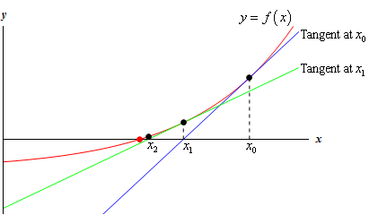
Step 1: Choose an Initial Guess

Begin by estimating an approximate value for the root (x_{0}​) close to where the equation might equal zero.

Step 2: Apply the Iterative Formula

Calculate subsequent points (\(x_{n+1}\)​) using \(x_{n}\)​ and evaluate f(x) and its derivative \({f}' (x)\).

For example, solving \(f(x)=x^{2}−2=0\):

Start with \(x_{0}​=1.5\).

First iteration:

\(x_{1}​=1.5−\frac{1.5^{2}-2 }{2(1.5)} =1.41667\)

Repeat until convergence.

Step 3: Determine Convergence

Continue iterations until x_{n}​ stabilizes, indicating the approximation of a root. 

Real-World Applications of Quadratic Equations

Quadratics in Physics

Quadratic equations form a cornerstone of modern physics, providing models of many natural phenomena:

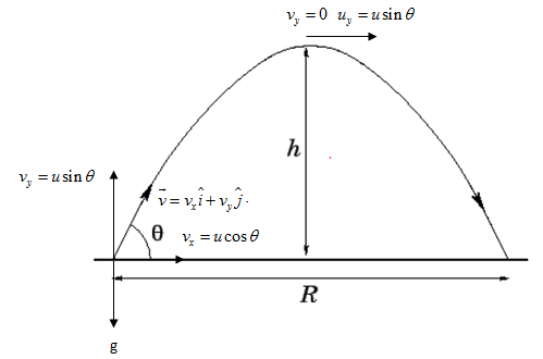
Projectile Motion: Projectile height is an essential concept in ballistics and sports physics, determined by solving this quadratic: \(h(t)=−\frac{1}{2} ​gt^{2}+v_{0}​t+h_{0}\). Solving this quadratic will reveal either when an object reaches maximum height or hits ground, giving us time estimates. For instance, solving it reveals when it reaches maximum height or hits bottom.

Optics: Quadratic equations used in optics design describe parabolic mirrors and lenses, making their creation essential in developing telescopes, cameras, and lasers. By solving such equations, scientists are able to accurately forecast trajectories, optimize devices, and simulate physical interactions necessary for technological innovation.

Economic and Optimization Problems

Quadratic equations play a critical role in economics and resource optimization:

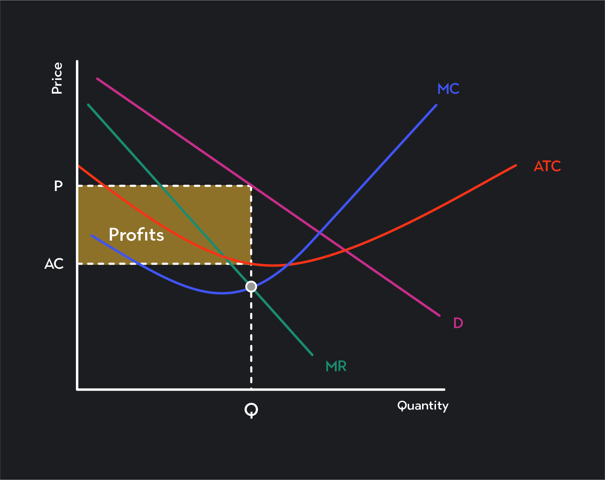
Profit Maximization: Quadratics model revenue and cost curves, enabling businesses to find profit-maximizing prices or production values. For example, if profit is expressed as \(P(x)=−x^{2}+50x−200\), solving the equation optimizes output.

Quadratic equations play an invaluable role in optimizing problems across industries by providing efficient resource allocation, cost reduction, and operational efficiencies, thus making quadratics an essential tool.

Conclusion

Mastery of quadratic equations builds a strong foundation not only in algebra but also in analytical thinking. Whether through factoring, completing the square, using the quadratic formula, or relying on graphical or numerical methods, each approach has its own strengths.

By exploring these techniques deeply, students and professionals can confidently solve diverse mathematical problems and apply their knowledge across disciplines.

Reference:

https://tutorial.math.lamar.edu/classes/calci/newtonsmethod.aspx

https://www.ga-ccri.com/can-a-neural-net-learn-the-quadratic-formula

https://github.com/aditeyabaral/gpython