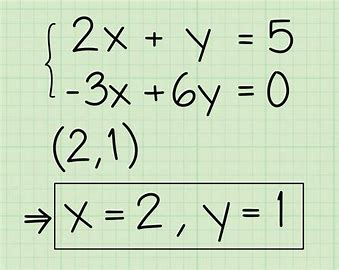
How to Solve a System of Equations?

What Is a System of Equations?

Definition

At its core, a system of equations refers to any set of two or more algebraic equations involving similar variables that must all come true simultaneously. When solving such systems of equations, the goal should be finding variable values that make all equations true. For a simultaneous example, consider the following system of two equations:

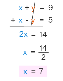
x+y=10 and x−y=4

Here, the variables x and y are shared across both equations. The solution to this system is x=7 and y=3, as these values satisfy both equations when substituted.

Importance

Systems of equations are at the core of algebra because they allow us to solve relationships among multiple quantities and quantities that depend on one another. They're more than abstract ideas: systems of equations provide practical tasks like allocating resources or determining forces on an object by mastering techniques for solving them efficiently and applying our knowledge across many areas that require optimization or problem-solving.

Types of Systems of Equations

Systems of equations can be classified in multiple ways, primarily based on the number of solutions and the type of equations involved.

Classifications Based on the Number of Solutions

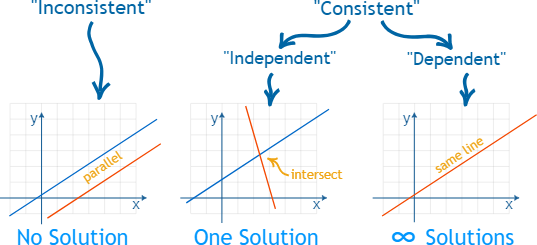
Unique Solution

A system of equations has a unique solution when there is exactly one set of variable values that satisfies all the equations. For instance:

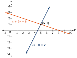
2x+y=6 and x−y=2

Graphically, this corresponds to two lines intersecting at a single point x=2,y=2. Unique solutions are critical in modeling problems with fixed constraints, such as budgeting within a specific financial limit.

No Solution

A system without an obvious solution often results when all its equations represent parallel lines which never cross each other; there simply cannot be any values which make all equations true at any one time. For example:

x+y=3 and x+y=5

These lines are parallel and distinct, indicating that the system has no solution.

Infinite Solutions

When a system has infinitely many solutions, the equations essentially describe the same line. For example:

x+y=3 and 2x+2y=6

Both equations represent one line, with every point on it representing a solution for the system. Such instances arise in scenarios with redundant constraints or incomplete information among them.

Linear vs. Nonlinear Systems

Linear Systems

Linear systems are systems in which all the equations are linear, meaning they form straight lines in a two-dimensional graph. Such systems take the general form:

Ax+By=C

Linear systems are crucial because their solutions can be reliably and quickly solved via substitution, elimination, or matrices.

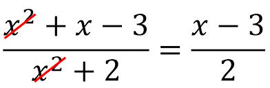
Nonlinear Systems

Nonlinear systems, on the other hand, involve at least one equation that is not linear—these might involve exponents, roots, or other complex relationships. For example:

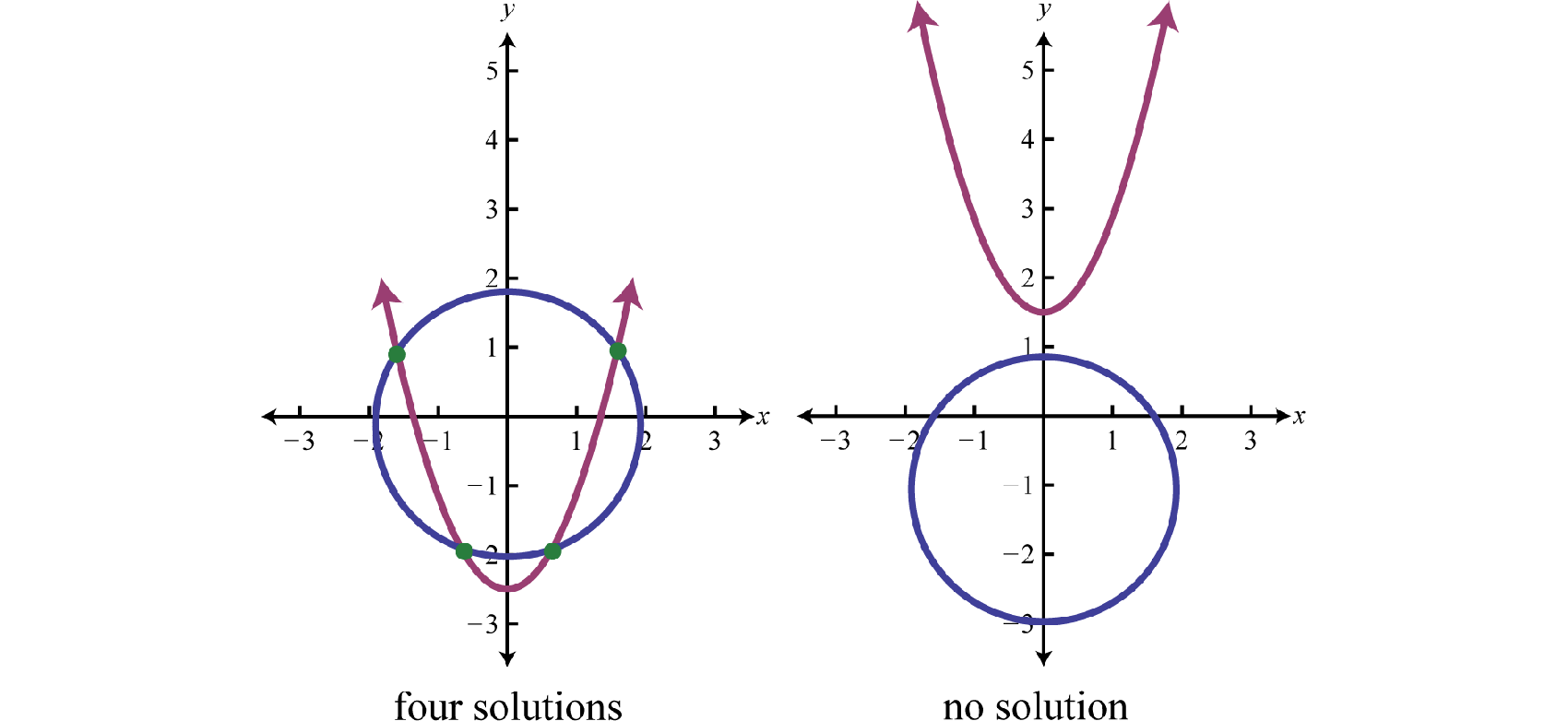
\(x^{2} + y^{2} =25\) and y=2x

These equations represent a circle and a line, respectively. Solving nonlinear systems often requires numerical methods, such as Newton's method or iterative approximation. Nonlinear systems are more challenging because the relationships between variables are more complex, and solutions may involve multiple intersections or no intersections at all.

Methods for Solving Systems of Equations

Now that we understand what systems of equations are and the types of solutions they can have, let's explore detailed techniques for solving them.

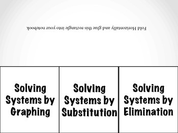
Substitution Method

The substitution method involves isolating one variable in one equation and substituting that expression into the other equation to reduce it to a single-variable equation.

Step 1: Isolate One Variable

Select an equation and isolate one variable by expressing it in terms of the other. For example, from the equation y=2x+1, y has been isolated in terms of x.

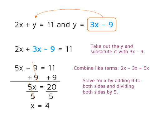
Step 2: Substitute into the Second Equation

Replace this expression for y in the second equation. For example, if the second equation is x+y=7, substitute y=2x+1 to get:

x+(2x+1)=7

Step 3: Solve the Single-Variable Equation

Simplify the equation to solve for x:

3x+1=7⟹3x=6⟹x=2

Step 4: Back-Substitute

Plug x=2 into the first equation to solve for y:

y=2(2)+1=5

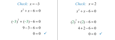
Step 5: Verify the Solution

Plug in x=2 and y=5 into the initial equations to verify the solution.

x+y=7⟹2+5=7,and y=2x+1⟹5=4+1

Thus, the solution is x=2,y=5. Substitution is most effective when one of the equations is already partially solved for a variable.

Elimination Method

The elimination method is an efficient approach to solving systems of equations by canceling out one variable.

Step 1: Adjust the Coefficients

Multiply one or both equations to make the coefficients of one variable equal in magnitude but opposite in sign. For example, consider the equations:

2x+3y=12 and 4x−y=10

Multiply the second equation by 3 to match the y-coefficients:

2x+3y=12 and 12x−3y=30

Step 2: Add or Subtract

Add the two equations to eliminate y:

(2x+3y)+(12x−3y)=12+30⟹14x=42

Solving gives x=3.

Step 3: Solve for the Remaining Variable

Substitute x=3 into the first equation:

2(3)+3y=12⟹6+3y=12⟹3y=6⟹y=2

Step 4: Verify the Solution

Always check the solution in both original equations to ensure accuracy. The solution to this system is x=3,y=2.

Tip: Look for coefficients that can easily be scaled (e.g., doubles, triples) to streamline the elimination process.

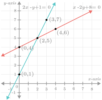
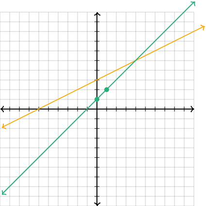
Graphical Method

The graphical method involves plotting each equation on a coordinate plane and identifying their intersection points. This method provides an intuitive, visual understanding of the system.

Steps

Convert all equations to slope-intercept form (y=mx+b).

For instance, 2x+y=6 becomes y=−2x+6.

Plot each equation on a coordinate plane. The slope (m) determines the line's steepness, and the y-intercept (b) determines where it crosses the y-axis.

Identify the intersection point(s), which represent the solution(s) to the system.

Example

For y=−2x+6 and y=\frac{1}{2} x+3, graphing will show the lines intersect at x=2,y=4. This is the system's solution.

Cross-Multiplication Method

Definition

The cross-multiplication method provides an indirect, formula-based approach to solving systems of two linear equations with two unknowns. It does away with step-by-step calculations by directly applying formulae derived from the determinant matrix as directly applied rules of thumb.

Steps

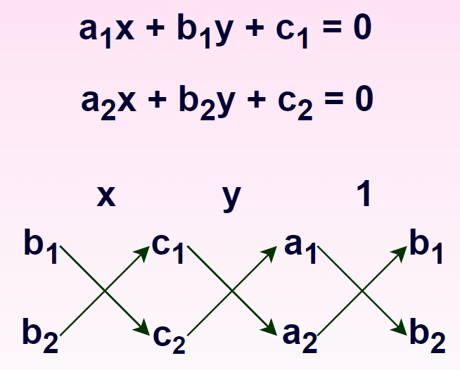
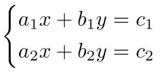
For two equations:

\(m_{1} ​x+n_{1} ​y+p_{1} = 0\) and \(m_{2} x+n_{2} ​y+p_{2} = 0\)

The formulas to solve for x and y are:

\(x/(n_{1}​ p_{2}​−n_{2}​ p_{1}​)=−y/(m_{1}​ p_{2}​​−m_{2}​ p_{1}​​)=1/(m_{1}​ n_{2}​−m_{2}​ n_{1}​)\)

Solve for x using:

\(x=(n_{1}​ p_{2}−n_{2} ​p_{1}​) / (m_{1}​ n_{2}​−m_{2} ​n_{1}​)\)

Solve for y using:

\(y=(p_{1}​ m_{2}​−p_{2}​ m_{1}​)/(m_{1}​ n_{2}​−m_{2}​ n_{1}​)\)

Example Methodology

For the equations:

x+y=5 and 2x−3y+7=0

With coefficients \(a_{1} =1, b_{1} =1, c_{1} ​=−5\) and \(a_{2} ​=2, b_{2} ​=−3, c_{2} ​=−7\), use the formulas above to compute x and y. This method is effective when equations are explicitly represented in standard form.

Matrix Method

Definition

The matrix method provides a universal approach for solving systems of linear equations, especially in higher dimensions. The system of equations is rewritten in the form AX=B, where:

A=Coefficient Matrix,X=Variable Matrix,B=Constant Matrix.

For example, the system:

2x+3y=6 and x−2y=3

can be written as:

\(\begin{bmatrix} 2& 3\\ 1 &-2\end{bmatrix} \begin{bmatrix} x\\y\end{bmatrix}=\begin{bmatrix} 6\\3\end{bmatrix}\)

Steps

Express the System in Matrix Form

Use AX=B, where A is the coefficient matrix, X is the variable column matrix, and B is the constants column matrix.

Find the Inverse of the Coefficient Matrix A:

Compute \(A^{-1}\) :

\(A^{-1} = \frac{1}{det(A)} ​\begin{bmatrix} d & -b\\ -c&a\end{bmatrix}\)

For systems where\(det(A) \ne\) 0, calculate \(X=A^{-1}B\).

Solve for Variables: Use matrix multiplication to calculate X, giving the values of x and y.

Modern Tools

Programs like Python (NumPy), MATLAB, and Excel can handle larger matrices efficiently, providing quick solutions for systems with more equations and unknowns, which are challenging to compute manually.

How to Choose the Right Method

Suitability of Each Method

Each method for solving systems has its own strengths and is best used in certain circumstances:

Substitution Method: Substitution can quickly reduce a two-variable problem to just one variable equation by quickly replacing one variable with the others and quickly solving for them all at the same time. For instance, with equation y=2x+3, it becomes easy to combine these into just one-variable problem through substitution.

Elimination Method: Elimination can be most effectively utilized when coefficients can easily and quickly be aligned or quickly altered to reach equilibrium; for instance, systems like 2x+5y=12 and 4x+5y=20 are ideal candidates as their y terms cancel out after subtraction, making elimination an attractive solution.

Graphical Method: Provides a visual understanding of solutions but may become inapplicable when dealing with complex systems that involve decimals or fractions.

Matrix Method: Ideal for large systems involving three or more variables, the matrix approach helps tackle problems in an organized and efficient manner.

Original Decision Framework

When choosing a method, consider:

Structure of the System

Look for symmetries or simplified forms.

If one variable already has equal coefficients, use elimination.

If one variable can be isolated neatly, opt for substitution.

Size of the System

For small systems, manual methods (substitution/elimination) work fine; for larger ones, rely on matrices or numerical solvers.

Requirement for Precision

If exact solutions are needed, avoid graphical methods unless backed by software tools.

Common Mistakes and How to Avoid Them

Arithmetic and Algebraic Errors

A common issue when solving systems of equations is simple arithmetic errors, such as mismanaging the signs during addition or subtraction, forgetting to distribute a coefficient, or mishandling fractions.

Solution

To avoid errors, write out all steps clearly and verify calculations at each stage. For instance, when solving:

2x+3y=6 and 4x−y=10

make sure to deal consistently with signs: multiplying one equation by -1 must affect the entire equation.

Graphing Mistakes

When plotting lines or determining an intersection point using graphing techniques, there can be room for error when plotting them out and creating solutions - even small inaccuracies can lead to incorrect solutions being presented as answers.

Remedy

Always use graphing calculators or software like Desmos or Microsoft Excel when visualizing systems. A plotted graph can reveal whether the lines intersect, run parallel, or overlap completely, offering insights beyond precise coordinates.

Mistakes in Matrix Solutions

The matrix method presents special difficulties, particularly for near-singular matrices whose det(A) approaches zero; they produce unreliable inverses and therefore make the system unfeasible for use.

Solution

Numerical methods or iterative techniques may be needed. Also, Check for close determinant values to zero. Use computational tools like NumPy (Python) that automatically flag any unconditioned matrices.

Advanced Techniques for Complex Systems

Iterative Numerical Methods

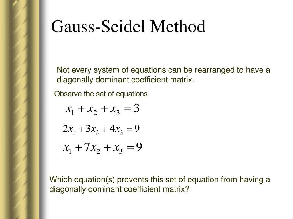
For nonlinear or large-scale linear systems, iterative methods such as the Newton-Raphson Method or the Gauss-Seidel Method are useful. These approaches repeatedly approximate solutions to improve accuracy.

Gauss-Seidel Method

This iterative method solves one variable at a time using approximations from previous iterations, continuously refining guesses.

Newton's Method for Nonlinear Systems

If your system contains equations like \(x^{2} + y^{2} =25\) and y=2x, Newton's Method employs derivatives to seek approximate solutions iteratively.

These techniques may require extensive computation power but are indispensable when approaching engineering and physics problems with complex solutions that cannot easily be expressed using simple languages.

Enhanced Use of Technology

Modern technology plays an essential role in solving complex systems. Python libraries such as SymPy and NumPy offer real-time computation for even large systems; tools such as MATLAB can manage matrices, execute iterative methods and construct three-dimensional visual graphs for even further visualization of data sets.

Applications in Real Life

Key Domains

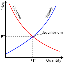
Economics 

Systems of equations model supply and demand curves, budgeting, and optimization challenges. For instance, finding the equilibrium price in a market requires solving two demand and supply equations.

Physics

Solve for forces in mechanical systems, as described by Newton's laws. For example, a system involving F=ma and v=u+at relates force, mass, and acceleration to velocity.

Business and Logistics

Systems are frequently used to optimize production schedules, minimize expenses, and allocate resources.

Problem Modeling Framework

Define Variables

Begin by identifying what x, y, and other variables represent in the problem.

Establish the System

Write equations that capture the constraints of the problem.

Select a Method

Choose a solving method based on problem complexity (e.g., small systems: substitution; large systems: matrix/numerical approaches).

Verify the Solution

Ensure the results align with real-world constraints and interpret the outcomes meaningfully.

Conclusion

Solving systems of equations is an essential skill with diverse applications across fields like economics, engineering, and physics. By understanding different kinds of systems (unique or none) with solutions--none or infinite--and using appropriate methods like substitution or elimination to get to unique or none solutions as quickly and accurately as possible using modern computational tools like Python's NumPy or MATLAB, we can ensure accuracy and efficiency even for complex or nonlinear systems; systems of equations provide us a powerful way of modeling real-world scenarios allowing us to analyze relationships better optimize decisions more confidently while solving practical challenges with ease!

Reference：

https://www.simplilearn.com/tutorials/excel-tutorial/data-analysis-excel

https://www.mdpi.com/2078-2489/11/4/193

https://www.statology.org/predictions-regression/