What is a Matrix?

Understanding the Basics of Matrices  

Before engaging in complex operations or applications, it's vitally important to learn about matrices' basic structure and foundational concepts. Here, you will explore their formal definition, interpretation of its elements, and relationship to real-world data systems.

Definition of a Matrix and its Order

Put simply, a matrix is a rectangular array of numbers organized into rows (horizontal entries) and columns (vertical entries). All the numbers or values inside the matrix are called elements. Each number is placed systematically under specific indices. Mathematically, a matrix is represented as:  

\(A = \begin{bmatrix} a_{11} & a_{12} & \dots & a_{1n} \\ a_{21} & a_{22} & \dots & a_{2n} \\ \vdots & \vdots & \ddots & \vdots \\ a_{m1} & a_{m2} & \dots & a_{mn} \end{bmatrix}\)

Here:  

- \(A\): The name of the matrix (capital English letter).  

- \(a_{ij}\): The element of matrix \(A\) at row \(i\) and column \(j\).  

- \(m\): The number of rows in the matrix.  

- \(n\): The number of columns in the matrix.  

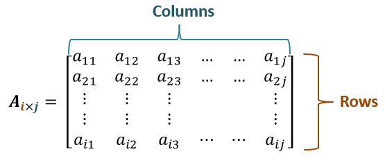
The order of the matrix is denoted as \(m \times n\), representing the number of rows and columns. For instance, a matrix \(A\) with 2 rows and 3 columns is said to have an order \(2 \times 3\).  

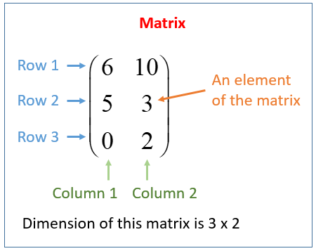
Rows, Columns, and Elements

Let’s break down these essential components:

- Rows: Rows in a matrix are the horizontal lines of elements. For matrix \(A\) of order \(m \times n\), the \(i\)-th row is written as \([a_{i1}, a_{i2}, \dots, a_{in}]\). 

- Columns: Columns in a matrix are the vertical stacks of elements. For matrix \(A\), the \(j\)-th column is \([a_{1j}, a_{2j}, \dots a_{mj}]^T\), where \(T\) represents transpose.

- Elements: Each individual number in the grid is called an element and is uniquely identified by its position \((i, j)\) within the matrix. For example, in a \(2 \times 3\) matrix \(B = \begin{bmatrix} 1 & 2 & 3 \\ 4 & 5 & 6 \end{bmatrix}\), \(b_{23} = 6\) because it is the element in the 2nd row and 3rd column.

Real-world Analogy of Matrices

Imagine using spreadsheets like Microsoft Excel. A spreadsheet is an excellent analogy for understanding matrices, as it is similarly divided into rows and columns, with each cell containing one value. For instance:

This table can be represented as a \(3 \times 4\) matrix, where each cell becomes an element. Such systems are useful in managing structured data across industries like finance, business, and logistics.

Types of Matrices

Matrices can come in different forms, each having its own specific structure and properties. Understanding them is vital as each type serves a distinct role when applied mathematical computations or applied across fields.

Classical Types of Matrices

Some of the commonly encountered matrices include:

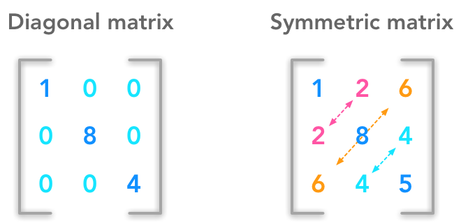
Symmetric Matrix

A square matrix \(A\) is symmetric if the element \(a_{ij}\) equals the corresponding element \(a_{ji}\). In other words, \(A = A^T\) (where \(A^T\) is the transpose of \(A\)). An example is:

\(A = \begin{bmatrix} 1 & 2 & 3 \\ 2 & 4 & 5 \\ 3 & 5 & 6 \end{bmatrix}\)

Here, notice that \(a_{12} = a_{21} = 2\), \(a_{13} = a_{31} = 3\), and so on. Symmetric matrices play a significant role in optimization problems and eigenvalue-related computations.

Skew-Symmetric Matrix

For a square matrix \(A\) to be skew-symmetric, the relation \(a_{ij} = -a_{ji}\) must hold for all \(i\) and \(j\), and its diagonal elements must always be zero. For example:

\(A = \begin{bmatrix} 0 & -3 & 2 \\ 3 & 0 & -7 \\ -2 & 7 & 0 \end{bmatrix}\)

Skew-symmetric matrices often arise in physics, particularly in representing rotational systems.

Diagonal Matrix

A diagonal matrix is characterized by all its non-diagonal elements being zero. For instance:

\(A = \begin{bmatrix} 4 & 0 & 0 \\ 0 & 5 & 0 \\ 0 & 0 & 6 \end{bmatrix}\)

Such matrices simplify computational operations like matrix inversion and finding eigenvalues.

Identity Matrix

The identity matrix, denoted by \(I\), is a special diagonal matrix where all diagonal elements are equal to 1, while all others are zero:

\(I = \begin{bmatrix} 1 & 0 & 0 \\ 0 & 1 & 0 \\ 0 & 0 & 1 \end{bmatrix}\)

The identity matrix acts as the multiplicative identity in matrix algebra, meaning \(IA = AI = A\) for any square matrix \(A\).

Advanced Types

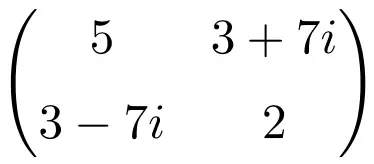
Hermitian Matrix

A matrix \(A\) is Hermitian if it is equal to its own conjugate transpose, i.e., \(A = A^\dagger\). For example:

\(A = \begin{bmatrix} 2 & i \\ -i & 3 \end{bmatrix}\)

Such matrices commonly appear in quantum mechanics.

Orthogonal Matrix

A square matrix \(A\) is orthogonal if its transpose equals its inverse, i.e., \(A A^T = A^T A = I\). These matrices are useful in transformations and rotations where unit length must be preserved.

Nilpotent Matrix

A square matrix \(A\) is nilpotent if there exists an integer \(p > 0\) such that \(A^p = 0\). For example:

\(A = \begin{bmatrix} 0 & 1 \\ 0 & 0 \end{bmatrix}, \quad A^2 = \begin{bmatrix} 0 & 0 \\ 0 & 0 \end{bmatrix}\)

Nilpotent matrices often arise in advanced linear algebra applications.

Relational Matrices

Relational matrices are particularly important in applied fields such as graph theory and data science. For example, an adjacency matrix represents the connections between vertices in a graph. If a graph has the vertices \(V_1, V_2,\) and \(V_3\), and edges connecting \(V_1\) to \(V_2\) and \(V_2\) to \(V_3\), the adjacency matrix is:

\(A = \begin{bmatrix} 0 & 1 & 0 \\ 1 & 0 & 1 \\ 0 & 1 & 0 \end{bmatrix}\)

Relational matrices simplify tasks like finding the shortest paths and analyzing networks in computer science.

Key Operations on Matrices

One of the essential reasons matrices are so widely used is because of the operations that can be performed on them. These operations are utilized for data manipulation: solving systems of equations, and performing transformations across various domains such as linear algebra and computer graphics.

Basic Arithmetic Operations

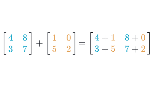
Matrix Addition and Subtraction

Matrices with the same dimensions can easily be added or subtracted element by element. If \(A\) and \(B\) are matrices of the same order \(m \times n\), then:

\((A + B)_{ij} = a_{ij} + b_{ij}, \quad (A - B)_{ij} = a_{ij} - b_{ij}\)

For example:

\(A = \begin{bmatrix} 1 & 2 \\ 3 & 4 \end{bmatrix}, \quad B = \begin{bmatrix} 5 & 6 \\ 7 & 8 \end{bmatrix}\)

Matrix addition gives:

\(A + B = \begin{bmatrix} 1+5 & 2+6 \\ 3+7 & 4+8 \end{bmatrix} = \begin{bmatrix} 6 & 8 \\ 10 & 12 \end{bmatrix}\)

Similarly, matrix subtraction would yield:

\(A - B = \begin{bmatrix} 1-5 & 2-6 \\ 3-7 & 4-8 \end{bmatrix} = \begin{bmatrix} -4 & -4 \\ -4 & -4 \end{bmatrix}\)

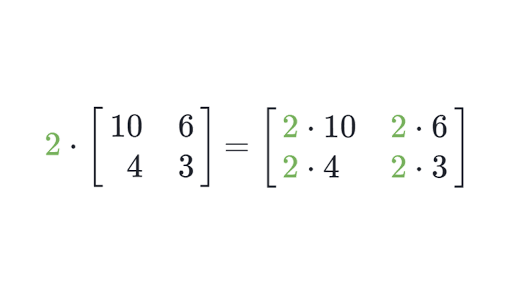
Scalar Multiplication

Multiplying a matrix by a scalar (a single number) involves simply multiplying each element of the matrix by that scalar. If \(k\) is a scalar and \(A\) is a matrix, scalar multiplication is defined as:

\((kA)_{ij} = k \cdot a_{ij}\)

For example, multiplying \(A = \begin{bmatrix} 1 & 2 \\ 3 & 4 \end{bmatrix}\) by \(k = 3\) gives:

\(3A = \begin{bmatrix} 3 \cdot 1 & 3 \cdot 2 \\ 3 \cdot 3 & 3 \cdot 4 \end{bmatrix} = \begin{bmatrix} 3 & 6 \\ 9 & 12 \end{bmatrix}\)

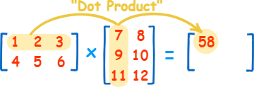
Matrix Multiplication

Matrix multiplication represents one of the fundamental operations in linear algebra. If \(A\) is an \(m \times n\) matrix and \(B\) is an \(n \times p\) matrix, then the product \(C = AB\) is defined as:

\(c_{ij} = \sum_{k=1}^n a_{ik} b_{kj}, \quad \text{for all } i = 1, \dots, m, \; j = 1, \dots, p\)

The resulting matrix \(C\) will have dimensions \(m \times p\). For example:

\(A = \begin{bmatrix} 1 & 2 \\ 3 & 4 \end{bmatrix}, \quad B = \begin{bmatrix} 5 & 6 \\ 7 & 8 \end{bmatrix}\)

Then the product \(AB\) is calculated as:

\(AB = \begin{bmatrix} (1)(5) + (2)(7) & (1)(6) + (2)(8) \\ (3)(5) + (4)(7) & (3)(6) + (4)(8) \end{bmatrix} = \begin{bmatrix} 19 & 22 \\ 43 & 50 \end{bmatrix}\)

Properties of Matrix Multiplication

- Associative property: \((AB)C = A(BC)\).

- Distributive property: \(A(B + C) = AB + AC\).

- Non-Commutative: \(AB \neq BA\) in general.

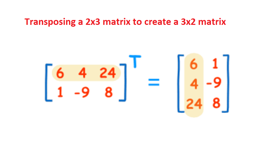
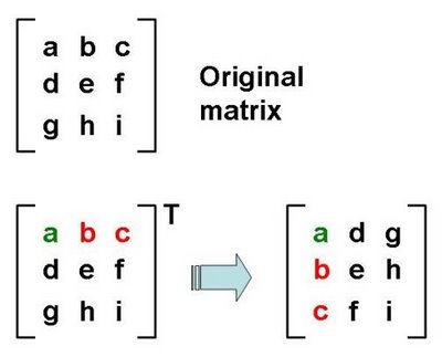
Matrix Transpose

The transpose of a matrix \(A\), denoted by \(A^T\), is formed by interchanging rows and columns of the matrix. Formally:

\((A^T)_{ij} = A_{ji}\)

For example, if:

\(A = \begin{bmatrix} 1 & 2 \\ 3 & 4 \\ 5 & 6 \end{bmatrix}\)

Then its transpose is:

\(A^T = \begin{bmatrix} 1 & 3 & 5 \\ 2 & 4 & 6 \end{bmatrix}\)

Matrix Interaction in Machine Learning

Matrix operations are at the core of machine learning algorithms. For instance:

1. Linear Regression: The weight vector \(\mathbf{w}\) in linear regression is calculated using matrix multiplication and inversion:

\(\mathbf{w} = (\mathbf{X}^T \mathbf{X})^{-1} \mathbf{X}^T \mathbf{y}\)

2. Neural Networks: Matrices are used to represent weights and activations. Given input \(\mathbf{x}\), weights \(\mathbf{W}\), and bias \(\mathbf{b}\), the output of a layer is computed as:

\(\mathbf{a} = \sigma(\mathbf{W} \mathbf{x} + \mathbf{b})\)

3. Gradient Descent: Gradients calculated during optimization are often represented and updated via matrix operations, making these procedures computationally efficient.

Determinants and Eigenvalues

Determinants and eigenvalues provide critical insights into the properties of matrices. These concepts are fundamental in solving linear systems, understanding geometry, and analyzing stability in dynamical systems.

Determinants of a Matrix

For a square matrix \(A\), the determinant (denoted as \(\det(A)\) or \(|A|\)) is a scalar value associated with the matrix. For a \(2 \times 2\) matrix:

\(A = \begin{bmatrix} a & b \\ c & d \end{bmatrix}, \quad \det(A) = ad - bc\)

For example:

\(A = \begin{bmatrix} 3 & 8 \\ 4 & 6 \end{bmatrix}, \quad \det(A) = (3)(6) - (8)(4) = 18 - 32 = -14\)

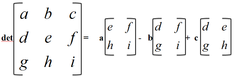
For a \(3 \times 3\) matrix, the determinant is:

\(A = \begin{bmatrix} a & b & c \\ d & e & f \\ g & h & i \end{bmatrix}, \quad \det(A) = a(ei - fh) - b(di - fg) + c(dh - eg)\)

Key Properties of Determinants

1. If \(\det(A) = 0\), then \(A\) is singular (not invertible).

2. For invertible matrices, \(\det(A^{-1}) = 1 / \det(A)\).

3. The determinant of the product of matrices satisfies \(\det(AB) = \det(A) \det(B)\).

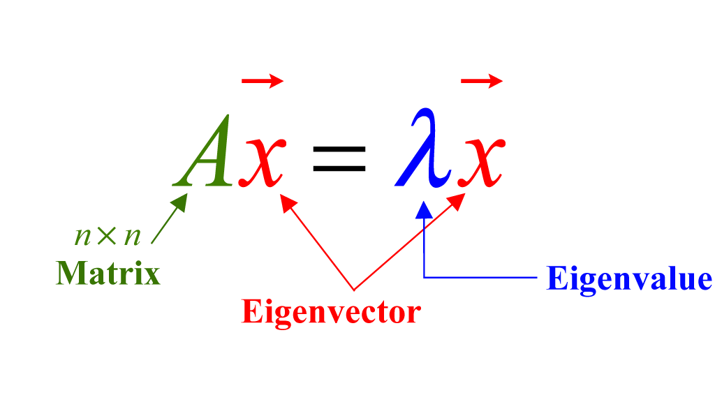
Eigenvalues and Eigenvectors

If \(A\) is an \(n \times n\) matrix, the eigenvalue equation is given by:

\(A \mathbf{v} = \lambda \mathbf{v}\)

Here:  

- \(\lambda\): An eigenvalue of the matrix \(A\).  

- \(\mathbf{v}\): A nonzero eigenvector corresponding to \(\lambda\).

The eigenvalues are found by solving the characteristic equation:

\(\det(A - \lambda I) = 0\)

Applications of Eigenvalues

- In mechanical systems, eigenvalues help predict oscillations and stability.

- In computer vision, eigenvalues are used to analyze features in image compression and facial recognition.

- In optimization, eigenvectors help construct principal components for Principal Component Analysis (PCA).

Applications of Matrices

Matrices are ubiquitous in addressing complex real-world problems because they can efficiently represent and process data in a structured manner. Their applications span across engineering, computer science, economics, physics, environmental science, and other fields.

Engineering and Computer Science

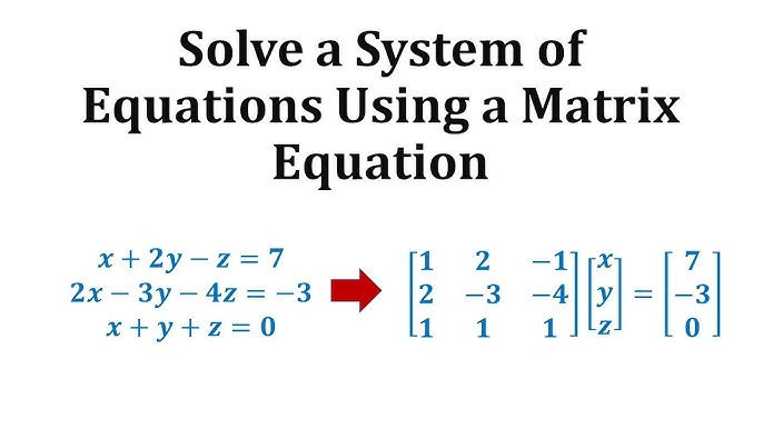
Systems of Linear Equations

One of the most important applications of matrices in engineering is solving systems of linear equations. Consider the system:

\(\begin{aligned} 2x + 3y &= 5 \\ 4x + y &= 11 \end{aligned}\)

This system can be represented in matrix form:

\(\begin{bmatrix} 2 & 3 \\ 4 & 1 \end{bmatrix} \begin{bmatrix} x \\ y \end{bmatrix} = \begin{bmatrix} 5 \\ 11 \end{bmatrix}\)

Let \(A = \begin{bmatrix} 2 & 3 \\ 4 & 1 \end{bmatrix}\), \(\mathbf{x} = \begin{bmatrix} x \\ y \end{bmatrix}\), and \(\mathbf{b} = \begin{bmatrix} 5 \\ 11 \end{bmatrix}\). Then the solution can be found as:

\(\mathbf{x} = A^{-1} \mathbf{b}\)

This representation allows for using computational tools like Gaussian elimination or LU decomposition to solve large systems efficiently.

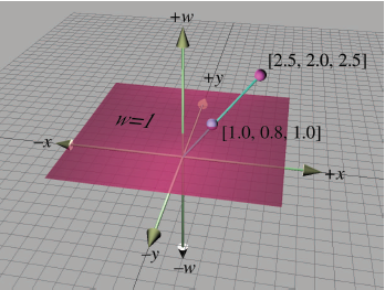
Computer Graphics and Transformations

In computer graphics, matrices are critical for performing transformations such as translation, rotation, scaling, and projection in 2D and 3D space. For example, to rotate a point \(\mathbf{v}\) in 2D by an angle \(\theta\), the rotation matrix \(R\) is:

\(R = \begin{bmatrix} \cos\theta & -\sin\theta \\ \sin\theta & \cos\theta \end{bmatrix}\)

The new point \(\mathbf{v}'\) after rotation is calculated as:

\(\mathbf{v}' = R \mathbf{v}\)

This concept forms the basis of games, animations and virtual reality; projection matrices use this principle for rendering 3D scenes onto 2D screens by simulating perspective.

Economics and Environmental Science

Input-Output Models

In economics, matrices model interactions between sectors in an economy using input-output analysis. For example:

\(\mathbf{x} = A\mathbf{y}\)

Where:

- \(\mathbf{x}\): Production output vector.  

- \(A\): Technology matrix, quantifying how sectors depend on each other.  

- \(\mathbf{y}\): Final demand vector.

This framework helps economists predict how changes in one sector (e.g., agriculture) may ripple through other sectors (e.g., manufacturing).

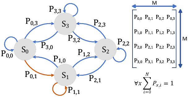
Environmental Modeling

Matrices can also play an invaluable role in environmental sciences for the analysis of ecological systems. Markov chains use them as representations of transition between states (for instance populations moving between habitats).

Consider a matrix \(P\), where \(p_{ij}\) is the probability of transitioning from state \(i\) to state \(j\). Repeated multiplications like \(P^k\) provide insights into the ecosystem's long-term equilibrium.

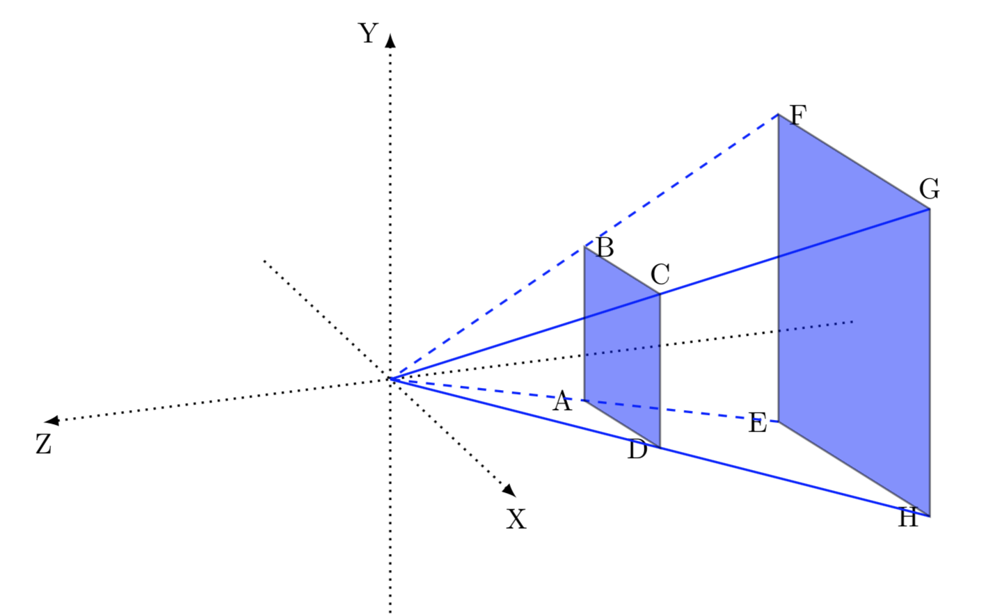
Perspective Mapping via Matrices

Matrices control perspective transformations in optics and cameras by manipulating image projections. In computer vision, a camera's 3D-to-2D mapping can be modeled as:

\(P = K [R | t]\)

Here:

- \(K\): Intrinsic matrix describing the camera's internal parameters (e.g., focal length).

- \(R\): Rotation matrix, modeling the camera's orientation.

- \(t\): Translation vector representing the camera's location in the scene.

This technique is essential for tasks like 3D model reconstruction, robotics navigation, and augmented reality applications.

Beyond Classical Matrices: Modern Innovations

As data becomes more complex in modern science and technology, traditional matrices are evolving into more sophisticated structures with new applications.

Sparse Matrices

Importance of Sparse Representations

In large datasets, the majority of matrix elements may be zeros. For example, in Internet connectivity matrices or social network graphs, most nodes are not directly connected. Representing such matrices in full form wastes memory and increases computational cost.

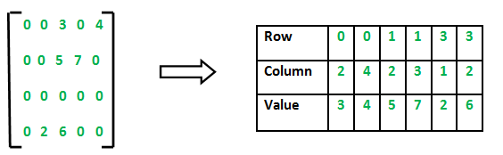
Sparse matrices efficiently store only the non-zero elements:

\(A = \{ a_{ij} : a_{ij} \neq 0 \}\)

Sparse matrix representations are widely used in machine learning (e.g., recommendation systems) and numerical simulations (e.g., finite element methods). CSR or CSC algorithms enable fast calculations while taking up minimal storage space.

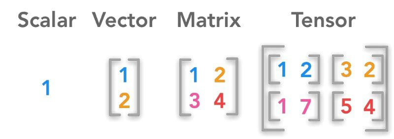
Tensor Matrices

Generalizing Matrices

Tensors are a generalization of matrices to higher dimensions. While a matrix is \(2D\) (\(m \times n\)), a tensor can operate in \(k\)-dimensions (\(n_1 \times n_2 \times \dots \times n_k\)). For example, a 3D tensor is represented as \(T \in \mathbb{R}^{n \times m \times p}\). 

Applications in Artificial Intelligence

Tensors are extensively used in AI, particularly in deep learning frameworks like TensorFlow and PyTorch, where they represent multi-dimensional data. For instance, during backpropagation in neural networks, tensors store:

1. Input Data: For images, a tensor might be \(\mathbb{R}^{B \times H \times W \times C}\), where \(B\): batch size, \(H, W\): height and width of the image, \(C\): channels (e.g., RGB).

2. Weights: Neural network layers assign weight tensors to learn patterns from data.

Tensor decomposition techniques like CANDECOMP/PARAFAC are used in recommender systems to understand patterns in high-dimensional data.

Frequently Asked Questions on Matrices

To further clarify common doubts about matrices, this section answers some of the most frequently asked questions.

Conceptual FAQs

What is the Transpose of a Matrix?

The transpose of a matrix involves converting its rows into columns and its columns into rows. For a matrix \(A\):

\(A = \begin{bmatrix} 1 & 2 \\ 3 & 4 \end{bmatrix}, \quad A^T = \begin{bmatrix} 1 & 3 \\ 2 & 4 \end{bmatrix}\)

How Do You Identify a Singular Matrix?

A matrix is singular if it is not invertible, i.e., \(\det(A) = 0\). For example:

\(A = \begin{bmatrix} 1 & 2 \\ 2 & 4 \end{bmatrix}, \quad \det(A) = (1)(4) - (2)(2) = 0\)

Practical FAQs

Why Are Matrices Important in Gaming and Animation?

Matrices can be used in gaming engines to effectively and efficiently transform objects, like object movement, scaling and rotation. Furthermore, they allow efficient calculations for lighting effects in 3D graphics graphics.

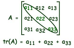
What is the Trace of a Matrix?

The trace of a square matrix is calculated as the sum of the elements on its main diagonal:

\(\text{tr}(A) = \sum_{i=1}^n a_{ii}\)

For example, if:

\(A = \begin{bmatrix} 3 & 5 \\ 7 & 8 \end{bmatrix}, \quad \text{tr}(A) = 3 + 8 = 11\)

Conclusion

Matrices are more than mathematical abstractions - they provide essential tools for organizing and processing data. From understanding basic matrix structures such as symmetric, diagonal, and identity matrices, to performing operations like addition, multiplication, and transposition, they offer an unrivaled framework for solving problems. Determinants and Eigenvalues offer additional insight, helping reveal hidden properties while solving real-world issues.

Beyond their classical uses, matrices and their modern extensions, like sparse matrices and tensors, play an increasingly vital role in cutting-edge fields like AI, computer vision, and financial modeling. Mastery of these versatile structures equips individuals with the analytical skills necessary to solve some of science and technology's most intriguing issues; mastering matrices provides individuals with analytical abilities necessary for solving some of its most interesting issues - be they modeling complex systems or diving into deep learning; mastery continues to spawn innovation!

Reference:

https://www.mdpi.com/2076-3417/14/1/306

https://arxiv.org/abs/2210.16182