What is Conditional Probability?

A Deeper Look into Conditional Probability

Definition and Importance

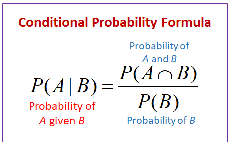
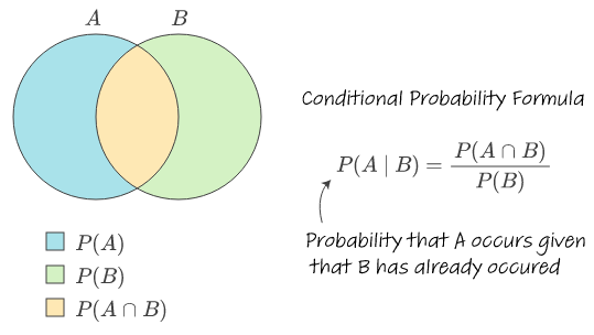
Conditional probability is expressed mathematically as P(A|B), which translates to "the probability of A occurring, given that B has occurred." The formula can be defined as:

\(P(A \mid B) = \frac{P(A \cap B)}{P(B)}, \quad \text{where } P(B) \neq 0\)

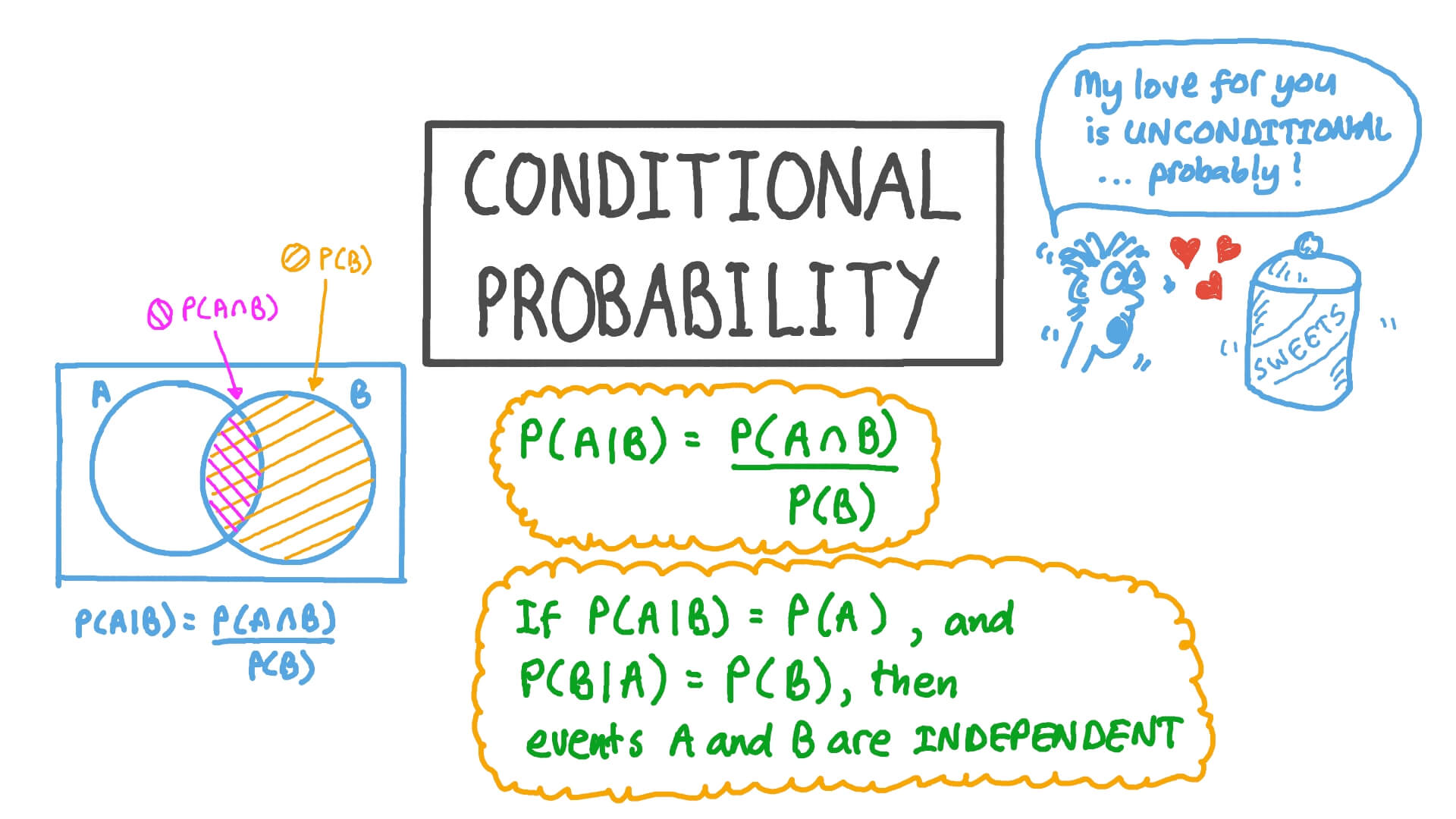
This shows how A (the dependent event) is determined by dividing its associated probability by that of B (the conditioning event).

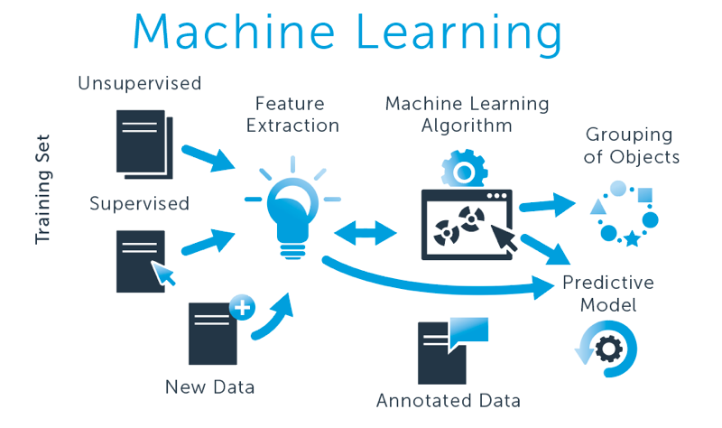
Conditional probability has far-reaching applications across industries and problems. Doctors rely on conditional probability when interpreting test data--assessing the probability that an illness exists given the results of diagnostic tests; financial analysts use conditional probabilities in predictive analytics models (e.g., predicting stock price movements based on sector performance); artificial intelligence/machine learning algorithms also use conditional probabilities efficiently in fine-tuning decision trees, improving classification systems and training predictive models efficiently.

Conditional probability is more than an abstract mathematical concept: its power lies in quantifying relationships. From tracking weather patterns and public health policies, to automating personalized e-commerce recommendations and automating personalized recommendations for products on sale online stores - conditional probability offers valuable foresight and optimization opportunities.

Everyday Examples

One way of understanding conditional probabilities is through familiar and straightforward scenarios:

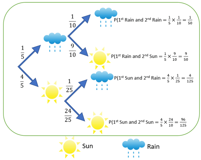
1. Weather Forecasting: Imagine being informed that there's only a 30% chance of heavy rainfall on any given day; when clouds cover up more of the sky than normal, meteorologists adjust this estimate to 70%! So now, rain becomes contingent upon cloudiness, creating P(Rain|Cloudy).

2. Medical Diagnostics: Assuming that when positive, certain medical tests indicate an 80% likelihood of disease presence; conditional probability can then be used to estimate this likelihood - P(Disease|Positive Test). This allows us to calculate disease prevalence probability given a particular outcome of testing.

3. Stock Market Analysis: Assuming stock A has a 60% chance of increasing in value, when investors observe high economic growth rates of, say, 5% or greater, this probability jumps up to 85%, and conditional probability helps market analysts calculate relationships such as P(A|High Growth).

Where Conditional Probability Shapes Decisions

Conditional probability's strength lies in its capacity to transform dependence between events into actionable insights. Machine learning practitioners use conditional probabilities as a basis for decision trees that reflect real-world decision-making processes influenced by earlier outcomes; urban planners employ crime analytics based on conditional probabilities to study patterns like an increase in burglaries occurring when street lighting decreases, for instance.

Businesses use predictive algorithms to improve customer behavior through tailored recommendations. For instance, an e-commerce platform might use your purchase of running shoes (Event B) as the basis for calculating whether you might buy fitness wear (Event A), responding accordingly and personalizing suggestions accordingly.

Conditional probability has become one of modern mathematics's revolutionary ideas due to its wide array of uses outside textbooks.

Key Concepts in Conditional Probability

Independent vs. Dependent Events

When exploring conditional probability, a fundamental concept revolves around differentiating independent and dependent events. This distinction is crucial for understanding how probabilities interact and why conditional probability becomes necessary in certain scenarios.

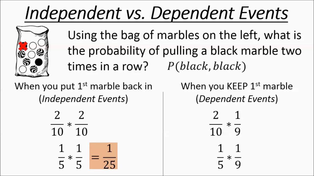
Independent Events

Two events are considered independent when the happening of one has no effect on the occurrence of the other. In such cases, the probability of one event happening does not depend on any prior knowledge of the other event. The mathematical relationship for independent events is:

\(P(A \cap B) = P(A) \cdot P(B)\)

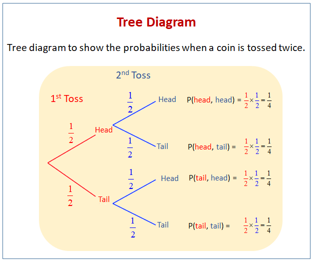
As an example, tossing a fair coin twice generates independent events, where the result of the first toss does not influence the outcome of the second. If the probability of flipping heads is \(P(\text{Head}) = 0.5\) for each toss, then the probability of flipping heads on both tosses is calculated as:

\(P(\text{Head, Head}) = P(\text{Head}) \cdot P(\text{Head}) = 0.5 \cdot 0.5 = 0.25\)

Dependent Events  

On the other hand, two events are dependent if the occurrence of one alters the probability of the other. Conditional probability is designed specifically to measure and handle such dependencies. For dependent events:

\(P(A \cap B) \neq P(A) \cdot P(B)\)

For example, consider drawing two cards from a standard deck of 52 cards without replacement. The likelihood of selecting an Ace (Event A) during the first draw is:

\(P(A) = \frac{4}{52}\)

Once an Ace is drawn, the composition of the deck changes, altering the probability of drawing a King (Event B) from the remaining 51 cards. This dependency makes Event B conditional on Event A.  

Real-Life Applications of Dependency

Dependency can be seen across various fields. For instance:

In epidemiology, models that predict infectious disease transmission frequently rely on dependent probabilities derived from interactions, vaccination rates, or population density changes as indicators of spreading.

Insurance actuaries use dependent probabilities to accurately gauge risk; for instance, when it comes to car accidents. They use factors like weather and road type conditions when making estimates such as how likely an incident might occur.

Hybrid Dependency in Real-World Models

Real-world scenarios often exhibit hybrid dependency - an approach we call multi-dependency - compared to either total dependence or independence. Take, for instance, the situation where a doctor conducts two diagnostic tests on one patient to evaluate their condition using different diagnostic tests whose results depend partially on those from the first as well as external influences like patient history or population data trends; mathematically speaking these situations necessitate advanced probabilistic models capable of representing these different dependencies simultaneously.

Formula and Notations of Conditional Probability

To properly compute conditional probabilities, it is essential to understand its formula and corresponding notations.

Standard Formula

The conditional probability formula originates from the connection between joint and marginal probabilities:

\(P(A \mid B) = \frac{P(A \cap B)}{P(B)}, \quad \text{where } P(B) \neq 0\)

Here:

- \(P(A \mid B)\) represents the conditional probability of Event A occurring given that Event B has already occurred.

- \(P(A \cap B)\) denotes the joint probability of both events A and B occurring at the same time.

- \(P(B)\) is the marginal probability of Event B.

This formula shows us that in order to calculate the conditional probability, we need to know two things:

1. The likelihood of both events occurring together.

2. The unconditioned probability of Event B.

For dependent events, the formula updates the base probability of Event A based on the new information related to Event B.

Probability Notation Explained

Understanding the symbols in conditional probability can be challenging, so let’s break them down here:

1. \(P(A)\): The simple or marginal probability of Event A occurring. This does not account for any other event and is calculated in isolation. Example: The probability of rolling a "4" on a fair six-sided die is:

\(P(4) = \frac{1}{6}\)

2. \(P(B \mid A)\): Represents the updated probability calculation. For example, the probability of landing on tails, having already thrown a weighted coin that favors heads:

\(P(\text{Tails} \mid \text{Weighted Heads})\)

3. \(P(A \cap B)\): Joint probability refers to the simultaneous occurrence of both events A and B. For instance, in a deck of cards, the probability of drawing a King and an Ace from two consecutive draws without replacement:

\(P(\text{King} \cap \text{Ace}) = P(\text{King}) \cdot P(\text{Ace} \mid \text{King})\)

Flexibility of Using the Formula

Conditional probability is incredibly versatile and has flexible applications across industries. For instance, financial analysts might calculate \(P(\text{Profit Increase} \mid \text{Positive Industry Growth})\) to judge stock performance.

Conditional Probability as a "Bayesian Framework"

Conditional probability provides the foundation for powerful frameworks like Bayes' Theorem and Bayesian inference, using conditional probability to constantly update predictions based on new evidence. For example, real-time traffic navigation apps adjust route recommendations \(P(\text{Best Route} \mid \text{Current Congestion})\) every time new traffic data arrives.

Conditional Probability vs. Other Types of Probabilities

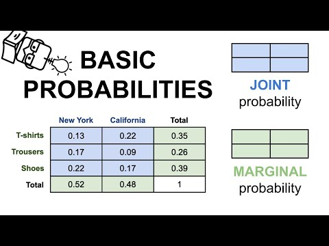
Probabilities are versatile tools that come in many forms depending on what is being measured. Conditional probability stands out because it introduces the concept of dependency, but to fully grasp its significance; we must explore how it contrasts with other types of probabilities, namely marginal and joint probabilities.

Marginal Probability

Marginal probability represents the likelihood of a single event happening on its own without taking any other events into account. It is the simplest type of probability and is often represented as \(P(A)\) or \(P(B)\). For example:

- The probability of picking an Ace from a standard deck of cards is:

\(P(\text{Ace}) = \frac{4}{52} = \frac{1}{13}\)

Marginal probabilities provide the cornerstone of probability theory. They are called marginal probabilities because their summations are over all possible outcomes of another random variable.

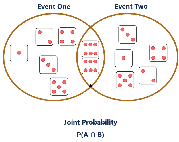
Joint Probability

Joint probability, on the other hand, describes the chance of two or more events happening at the same time. It is represented mathematically as \(P(A \cap B)\), where \(A\) and \(B\) are the events of interest. For example:

- The probability of drawing a red Ace from a standard deck of cards is:

\(P(\text{Red} \cap \text{Ace}) = \frac{2}{52} = \frac{1}{26}\)

Unlike marginal probability, joint probability looks at the overlap of two events. It assumes that both events happen together, and this overlap is particularly important when working with correlated outcomes.

Comparative Analysis: Marginal, Joint, and Conditional Probability

The primary distinction between these types of probability lies in how dependencies are treated:

1. Marginal Probability: Independent of other conditions or events, this measure represents absolute likelihood.

2. Joint Probability: Assesses the likelihood that two or more events will happen simultaneously and thus considers their interaction.

3. Conditional Probability: Conditional Probability is an extension of both methods, explaining how one event affects another one in relation to each other. Unlike joint probability, its primary concern lies with how an event changes its likelihood rather than co-occurrence itself.

The "Layered Cake" Model of Probability

An effective analogy for understanding these relationships is the "layered cake" model:

Base Layer: Marginal Probabilities that provide an understanding of individual outcomes as foundational concepts.

Middle Layer: Joint probabilities, represented as slices that interweave between layers to represent events that take place simultaneously;

Top Layer: Conditional probabilities that slice and dice the cake more precisely depending on available information.

Assume you're conducting analysis for an online store. Your base layer could consist of marginal probabilities for purchasing any item; your middle layer might look at simultaneous purchases (for instance buying both shoes and socks at once); finally your top layer might focus on specific dependencies (ie the likelihood of buying socks given that shoes had already been bought).

Taking an iterative approach helps contextualize conditional probability as an analytical tool which narrows focus while taking account of external knowledge in making informed decisions.

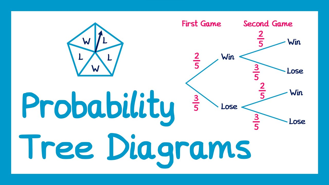
Tree Diagrams and the Multiplication Rule

Tree diagrams and the multiplication rule play essential roles in visualizing and simplifying multi-step probability calculations. Together, they provide clarity for solving more complex conditional probability scenarios.

How Tree Diagrams Work

A tree diagram is a branching visual representation used to map out the probabilities of sequential events systematically. Each branch represents a possible outcome, and by following pathway probabilities step by step, both simple and conditional probabilities can be calculated.

Example: Basic Tree Diagram

Suppose you are analyzing a two-step scenario: flipping a fair coin and then rolling a six-sided die. The outcomes can be mapped as follows:

1. Step 1: The coin outcomes (Heads or Tails) each have a probability of \(0.5\).

2. Step 2: For each branch (Heads or Tails), the die outcomes range from 1 to 6 with probabilities \(\frac{1}{6}\).

The tree would have 12 branches in total, each ending in a unique event, such as "Heads-3" or "Tails-5." Probabilities of specific outcomes can be calculated by multiplying probabilities along each branch.

Benefit of Visualization

Tree diagrams simplify probabilistic reasoning by breaking it into manageable steps. They allow us to visualize events' dependencies and reduce manual errors.

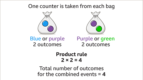
Incorporating the Multiplication Rule into Tree Diagrams

The Multiplication Rule links joint probabilities to conditional probabilities:

\(P(A \cap B) = P(A) \cdot P(B \mid A)\)

This formula is especially useful for calculating probabilities in sequentially dependent scenarios. For instance:

- Suppose a jar contains five red candies and three blue candies. If one candy is drawn without replacement, the probability tree diagram will feature the following:

- First Draw: Red (\(P(R_1) = \frac{5}{8}\)) and Blue (\(P(B_1) = \frac{3}{8}\)).

- Second Draw: Dependent probabilities for subsequent outcomes (e.g., \(P(R_2 \mid R_1)\)) adjust based on what was drawn first. These conditional probabilities capture the dependency between draws.

Real-Life Applications of Tree Diagrams and Multiplication Rule

In practice, tree diagrams often model:

- Medical Diagnoses: Calculating errors or successes of multi-stage tests.

- Investment Portfolios: Assessing step-by-step gains or losses across interdependent financial scenarios.

- Board Games: Designing player probabilities from multi-turn games (e.g., Monopoly).

Tree Diagrams as Probability Debugging Tools

Tree diagrams go beyond simply calculating probabilities - they also allow us to detect errors in reasoning. For instance:

Tree diagrams can assist with solving probability problems by helping model all possible paths correctly to ensure clarity and accuracy in calculations. They allow clarity over complexity.

Tree diagrams may prove particularly effective at diagnosing system failures by uncovering "forgotten branches," such as hardware malfunction, that would otherwise go undetected and distort total reliability calculations.

Thus, tree diagrams not only serve as computational aids but are also powerful conceptual tools for grasping probabilities across multiple steps.

Conditional Probability and Bayes' Theorem

Conditional probability serves as the foundation for Bayes' Theorem — a principle that allows us to reverse or update probabilities in light of new evidence.

Introduction to Bayes' Theorem

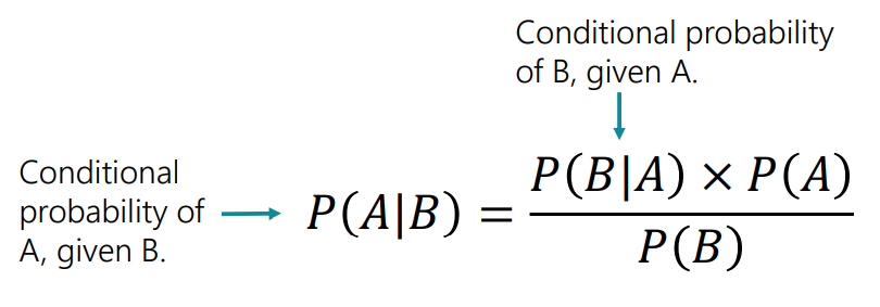
Bayes' Theorem mathematically reshapes conditional probability:

\(P(A \mid B) = \frac{P(B \mid A) \cdot P(A)}{P(B)}, \quad \text{where } P(B) \neq 0\)

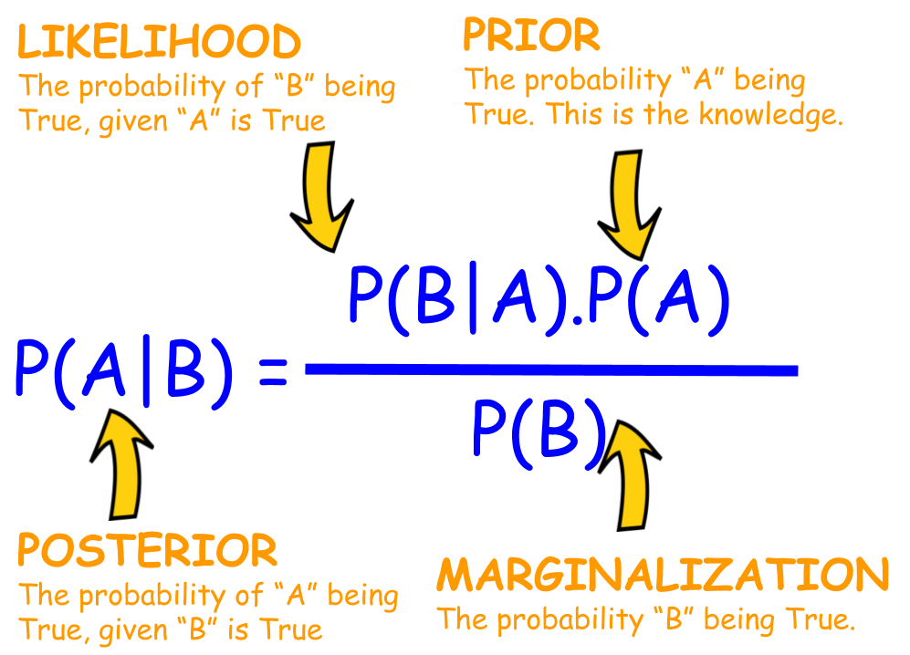
Where:

- \(P(A \mid B)\): The updated probability of \(A\) occurring given \(B\).  

- \(P(A)\): The prior or baseline probability of \(A\).

- \(P(B \mid A)\): The likelihood of \(B\) given that \(A\) has occurred.

- \(P(B)\): The marginal probability of \(B\) occurring at all.

The theorem is particularly powerful when direct calculations of \(P(A \mid B)\) are difficult, but related probabilities such as \(P(B \mid A)\) are easier to evaluate.

Practical Applications

Bayes' Theorem excels in a variety of real-world contexts:

Healthcare Diagnostics

Using \(P(\text{Disease} \mid \text{Positive Test})\) to assess the likelihood of having a disease given a positive result. By adjusting based on test accuracy (\(P(\text{Positive Test} \mid \text{Disease})\)) and disease prevalence (\(P(\text{Disease})\)), doctors can make better diagnoses.

Spam Filtering

Email algorithms predict the probability of an email being spam (\(P(\text{Spam} \mid \text{Suspicious Words})\)) by analyzing word frequencies.

Autonomous Driving

Systems estimate driving risks using Bayesian approaches where new evidence (\(B\)), like road conditions, continuously updates the probabilities of accidents (\(P(\text{Accident} \mid B)\)).

Beyond Static Updates

Bayes’ Theorem is also pivotal in dynamic systems. For example, weather forecasts are continually refined using streaming satellite updates. Probabilities based on initial models \(P(\text{Rain} \mid \text{Sky})\) are revised hourly based on new satellite data.

Bayesian Thinking in Artificial Intelligence  

The significance of Bayes' Theorem extends beyond mathematics into psychology and artificial intelligence (AI). Humans often struggle with accurate probability reasoning due to cognitive biases, but AI systems powered by Bayesian models excel at overcoming these limitations.

For example:

- Recommendation Engines: Netflix suggests movies using probabilities \(P(\text{Like} \mid \text{Genre Preferences})\) influenced by watching history.

- Spam Classifiers: Bayesian filters endure sophisticated spam patterns by continually learning \(P(\text{Spam} \mid \text{Tricky Scam Patterns})\) and adapting filters.

Bayes’ Theorem bridges past evidence with updated knowledge, helping algorithms make decisions in evolving environments faster and more accurately than human intuition.

Real-Life Applications of Conditional Probability

Conditional probability is more than just an academic concept; its real-world applications span across industries. From disease prediction to optimizing financial strategies, understanding dependencies between events has provided actionable insights that inform key areas of decision-making.

Healthcare and Diagnostics

In the medical field, conditional probability is a cornerstone of diagnostic analysis. Healthcare professionals routinely analyze patient test results to infer the likelihood of a disease given specific symptoms or test outcomes.

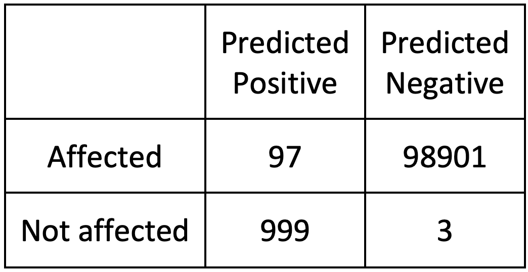
Example: Disease Diagnosis

Suppose a blood test for a disease has a 95% sensitivity (true positive rate) and an 85% specificity (true negative rate). If the disease's overall prevalence within the population is 1%, Bayes' Theorem can be used to calculate the probability of actually having the disease given a positive test result (\(P(\text{Disease} \mid \text{Positive Test})\)). This accounts for the test's accuracy and the disease's prevalence, guiding doctors to avoid a false sense of certainty in low-prevalence conditions.

Such computations are paramount during pandemics, where interpreting test results helps target containment measures effectively.

Financial Risk Management

The finance industry leverages conditional probability to quantify and mitigate market risks, calculate credit scores, and optimize investments. For example:

- Loan Defaults: Banks may assess the probability of a borrower defaulting on a loan (\(P(\text{Default} \mid \text{Bad Credit History})\)). By considering probabilities conditioned on credit history, income levels, and employment status, financial institutions create more reliable lending policies.

- Portfolio Risk Analysis: Investment firms calculate probabilities of stock performance under certain economic conditions, such as \(P(\text{Stock Rise} \mid \text{GDP Growth})\). This helps structure portfolios that hedge against dependencies.

Environmental Forecasting

Conditional probability is heavily used in environmental sciences to predict weather and natural disasters. For instance:

- Flood Prediction: Engineers and environmental scientists analyze the probability of floods (\(P(\text{Flood} \mid \text{Heavy Rainfall})\)) based on rainfall conditions and geographical factors.

- Climate Modelling: Estimations such as \(P(\text{Temperature Increase} \mid \text{Carbon Dioxide Levels})\) inform global policies on tackling climate change.

Conditional Probability in Decision Automation

One of the most cutting-edge applications of conditional probability is in autonomous decision-making systems. Algorithms in self-driving cars estimate risks dynamically. For instance:

- \(P(\text{Collision} \mid \text{Traffic Flow})\) allows onboard systems to predict and act on impending dangers based on real-time data.

- Intelligent systems also optimize delivery routes using conditional forecasts, such as \(P(\text{Delay} \mid \text{Rain in City X})\).

Across industries, the synthesis of probabilities conditioned on contextual data feeds into decision-making algorithms, automating tasks once governed by human discretion.

Complex Problems and Common Misconceptions

Conditional probability can be remarkably intuitive when applied to simple scenarios, but real-life situations often present challenges. Additionally, misconceptions surrounding conditional probability can lead to errors in analysis and decision-making.

Challenging Problems

Real-world issues in conditional probability often involve complex situations with multiple conditions interacting, necessitating careful setup and computation to ensure no crucial aspect is overlooked.

Example: Multi-Level Dependencies

Consider rolling three dice simultaneously and calculating the probability of getting at least one "6," provided the sum of the dice is odd. This problem introduces interdependencies that are not immediately obvious. Each dice roll affects the sum of the set (\(P(\text{Sum Odd})\)), and this, in turn, changes the probability for individual outcomes like rolling a "6." A step-by-step breakdown is required to avoid errors, dividing the problem into manageable conditional slices.

Example: Combined Events

Calculating probabilities of complex combinations like drawing two Aces followed by a King without replacement can be complicated in card games, which makes direct computation challenging.

Tree diagrams and systematic application of the formulas \(P(A \mid B)\) and \(P(B \mid A)\) become essential in these instances.

Misconceptions and Errors

Misconceptions regarding conditional probability arise frequently as a result of mixing it up with other types of probability or misunderstanding its relation to event dependence.

Interchanging Joint and Conditional Probabilities

Many errors stem from interpreting \(P(A \cap B)\) (joint probability) as \(P(A \mid B)\) or vice versa, resulting in flawed conclusions. This misconception often appears in areas like medical testing, where failing to differentiate between \(P(\text{Disease} \cap \text{Positive Test})\) and \(P(\text{Disease} \mid \text{Positive Test})\) could mislead diagnoses.

Assuming Independence Without Verification

A common mistake is to assume two events are independent when they are, in fact, dependent. For example, in analyzing market trends, assuming \(P(\text{Stock A Rise} \cap \text{Stock B Fall}) = P(\text{Stock A Rise}) \cdot P(\text{Stock B Fall})\) ignores potential dependencies between the two stocks, leading to incorrect forecasts.

Scenarios of Misused Conditional Probabilities

One frequently misused scenario involves confusion between correlation and causation. For example:

- Studies might suggest \(P(\text{Heart Disease} \mid \text{Alcohol Consumption})\) is high in certain demographics. However, interpreting this as causation could ignore shared dependencies, like \(P(\text{Heart Disease} \mid \text{Dietary Patterns})\), confounding analyses and policy recommendations.

Across domains, understanding the precise meaning and implications of conditional probabilities is critical to avoiding errors and biases that misuse the data.

Conclusion

Conditional probability is a practical and impactful concept that allows us to interpret the likelihood of events in the context of dependencies. Tools like Bayes' Theorem, tree diagrams, and the multiplication rule equip individuals and automated systems to make reliable predictions and informed decisions.

Conditional probability has numerous applications across healthcare, finance and AI that demonstrate its utility for solving real world issues and optimizing outcomes. Proper use requires distinguishing among independence, correlation and causation to avoid misinterpretations of conditional probability estimates.

Mastery of conditional probability is critical in an increasingly interdependent and data-driven world, helping individuals address uncertainties effectively while making rational, data-supported choices efficiently.

Reference:

https://www.amazon.com/Signal-Noise-Many-Predictions-Fail-but/dp/0143125087

https://plato.stanford.edu/entries/epistemology-bayesian/

https://stats.libretexts.org/Bookshelves/Introductory_Statistics/Inferential_Statistics_and_Probability_-_A_Holistic_Approach_(Geraghty)/05%3A_Probability/5.08%3A_Multiplicative_Rule_and_Tree_Diagrams