What Is Probability?

Probability permeates many aspects of our everyday lives, from weather forecasting to game odds. But what exactly is probability? Does it represent some intrinsic property of reality, or are humans simply using mental models of uncertainty as a form of defense against risk? In this article we dive deep into probability by exploring its definition, theoretical foundations, historical development, and practical applications; our aim being a complete picture of its importance across fields.

Definition

Basic Concepts

Probability, in its basic definition, measures the likelihood of something happening and quantifies uncertainty by providing a numerical value between 0 and 1, where 1 represents certainty and 0 represents impossibility. Probability draws heavily upon concepts associated with randomness and uncertainty inherent to both natural processes as well as human-made ones.

Introduction to Related Terms

Random Variable

Definition

Random variables are essential components of probability theory and statistics, providing us with different numerical values depending on the results of random experiments. There are two categories of random variables—discrete and continuous.

- Discrete Random Variable: A discrete random variable has finite or countable distinct values; examples may include the number of heads in 10 coin flips, defective items found within a batch, or customers entering a store within one hour.

- Continuous Random Variable: Continuous random variables have the ability to take on any number of values within their specified range, such as the height of people or times spent accomplishing specific tasks, temperatures at specific locations.

Examples

1. Discrete Random Variable: Consider rolling a six-sided die. The possible outcomes are 1, 2, 3, 4, 5, and 6. If we define a random variable \(X\) as the number showing on the die, \(X\) is a discrete random variable because it can only take on one of six specific values.

2. Continuous Random Variable: Consider measuring the time it takes for a computer to boot up. If we define a random variable \(Y\) as the boot-up time, \(Y\) is a continuous random variable because it can take on any value within a range, such as 0 to 60 seconds.

Properties

- Probability Mass Function (PMF): For a discrete random variable, the probability mass function \(P(X = x)\) gives the probability that the random variable \(X\) takes on the value \(x\).

- Probability Density Function (PDF): For a continuous random variable, the probability density function \(f_Y(y)\) gives the relative likelihood of the random variable \(Y\) taking on a specific value \(y\). The probability of \(Y\) falling within a specific interval is found by integrating the PDF over that interval.

- Cumulative Distribution Function (CDF): The cumulative distribution function \(F_X(x)\) for a random variable \(X\) gives the probability that \(X\) is less than or equal to \(x\). For a continuous random variable, it is the integral of the PDF.

Probability Distribution

Definition

Probability distributions provide a thorough description of how random variables' values are distributed over time, from discrete random variables with discrete probabilities associated with each possible value to continuous random variables where there may be several possible ranges to continuous random variables that contain more continuous probabilities within their ranges.

Types of Probability Distributions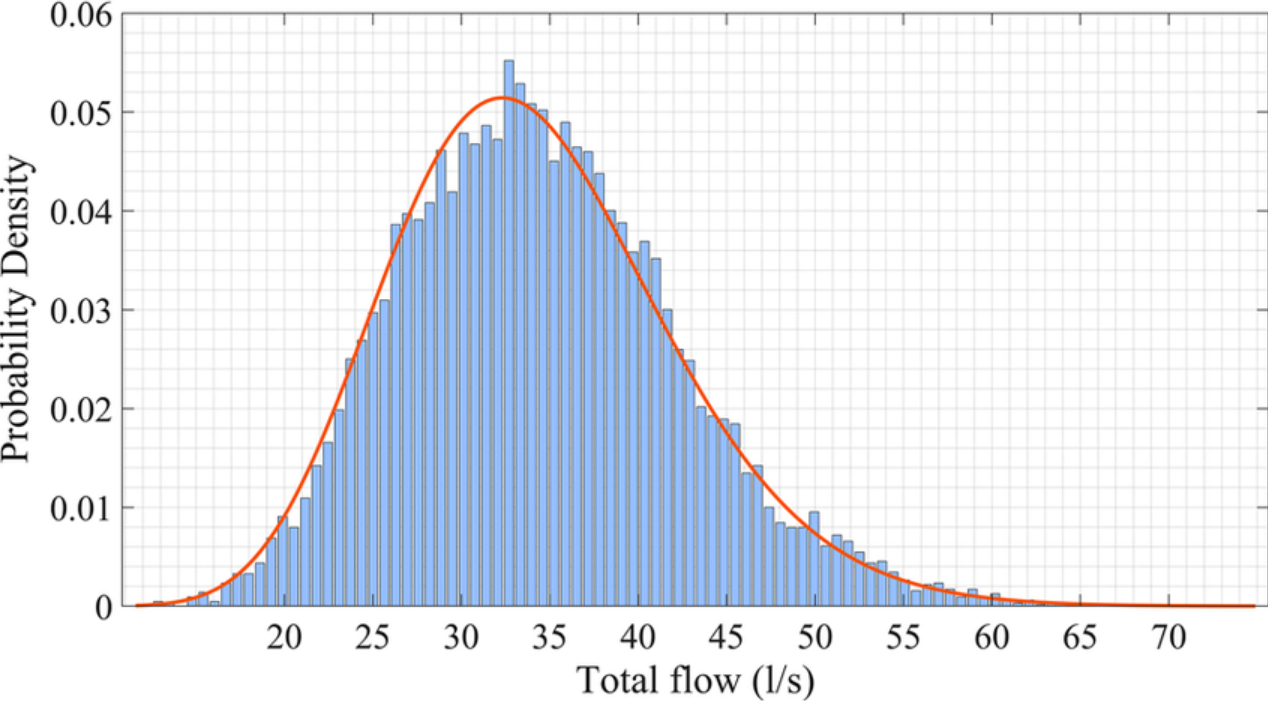

1. Discrete Probability Distributions:

- Binomial Distribution: Describes the number of successes in a fixed number of independent Bernoulli trials (e.g., flipping a coin \(n\) times).

- Poisson Distribution: Describes the number of events occurring in a fixed interval of time or space, given a constant average rate (e.g., the number of emails received per hour).

2. Continuous Probability Distributions:

- Normal Distribution: Also known as the Gaussian distribution, it describes a continuous random variable with a symmetric, bell-shaped curve. It is characterized by its mean (\(\mu\)) and standard deviation (\(\sigma\)).

- Exponential Distribution: Describes the time between events in a Poisson process, where events occur continuously and independently at a constant rate.

Examples

1. Binomial Distribution: Suppose we flip a fair coin 10 times. Let \(X\) be the number of heads obtained. \(X\) follows a binomial distribution with parameters \(n = 10\) and \(p = 0.5\).

2. Normal Distribution: Imagine an adult male population is normally distributed, with a mean height of 175 cm and a standard deviation of 10 cm; then any randomly sampled adult from this population follows this distribution when his height is measured.

Expected Value

Definition

The expected value (or mean) of a random variable is a measure of the center of its distribution. It represents the average value of the random variable over an infinite number of trials of the experiment. The expected value is denoted by \(E(X)\) for a random variable \(X\).

 Calculation

- Discrete Random Variable: The expected value \(E(X)\) of a discrete random variable \(X\) with possible values \(x_1, x_2, \ldots, x_n\) and corresponding probabilities \(P(X = x_i)\) is calculated as:

\(E(X) = \sum_{i=1}^{n} x_i \cdot P(X = x_i)\)

- Continuous Random Variable: The expected value \(E(Y)\) of a continuous random variable \(Y\) with probability density function \(f_Y(y)\) is calculated as:

\(E(Y) = \int_{-\infty}^{\infty} y \cdot f_Y(y) \, dy\)

Examples

1. Discrete Random Variable: Consider a die with faces numbered 1 through 6. The expected value of the outcome when rolling the die is:

\(E(X) = \sum_{i=1}^{6} i \cdot \frac{1}{6} = \frac{1 + 2 + 3 + 4 + 5 + 6}{6} = 3.5\)

2. Continuous Random Variable: Consider a continuous random variable \(Y\) representing the time (in hours) it takes to complete a task, with an exponential distribution with rate parameter \(\lambda = 1\). The expected value is:

\(E(Y) = \int_{0}^{\infty} y \cdot \lambda e^{-\lambda y} \, dy = \frac{1}{\lambda} = 1 \text{ hour}\)

Variance

Definition

Variance is a measure of dispersion or spread between values in a random variable and their expected values and quantifies by how much these vary from them. The variance of a random variable \(X\) is denoted by \(\text{Var}(X)\).

Calculation

- Discrete Random Variable: The variance \(\text{Var}(X)\) of a discrete random variable \(X\) with expected value \(E(X)\) is calculated as:

\(\text{Var}(X) = E[(X - E(X))^2] = \sum_{i=1}^{n} (x_i - E(X))^2 \cdot P(X = x_i)\)

- Continuous Random Variable: The variance \(\text{Var}(Y)\) of a continuous random variable \(Y\) with expected value \(E(Y)\) is calculated as:

\(\text{Var}(Y) = E[(Y - E(Y))^2] = \int_{-\infty}^{\infty} (y - E(Y))^2 \cdot f_Y(y) \, dy\)

Examples

1. Discrete Random Variable: Consider the same die example. The expected value is 3.5. The variance is calculated as:

\(\text{Var}(X) = \sum_{i=1}^{6} (i - 3.5)^2 \cdot \frac{1}{6} = \frac{1}{6}[(1 - 3.5)^2 + (2 - 3.5)^2 + \ldots + (6 - 3.5)^2] = 2.92\)

2. Continuous Random Variable: For the exponential distribution example with rate parameter \(\lambda = 1\), the variance is:

\(\text{Var}(Y) = \int_{0}^{\infty} (y - 1)^2 \cdot e^{-y} \, dy = 1\)

If you have any questions about these examples, you can consult online tutors at UpStudy's Ask Tutors.

Probability Tree Diagram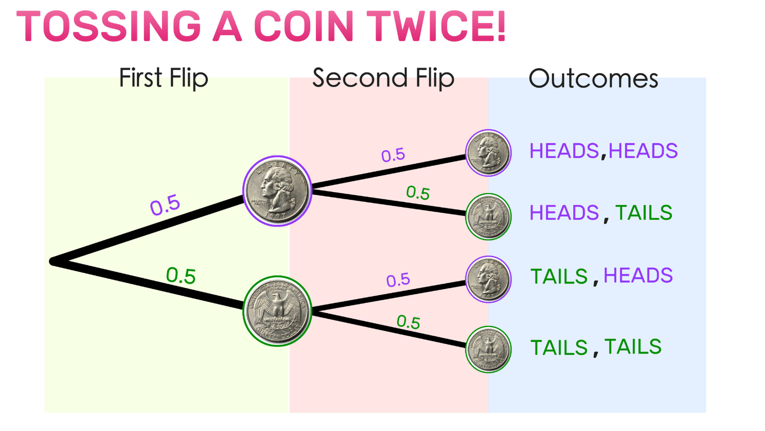

Probability tree diagrams provide a visual depiction of all possible outcomes of an experiment and their associated probabilities, making them especially helpful when handling complex experiments with multiple steps or events. Each branch in a probability tree represents one outcome with associated probabilities to help visualize sample space and calculate composite events' probabilities more quickly and effectively.

Consider, for instance, an experiment in which we flip a coin and roll a die; its probability tree diagram would consist of two initial branches for coin flips (heads or tails) followed by six additional ones representing die rolls (1 through 6). This allows us to easily calculate combined events, such as getting heads first before rolling 3! This diagram allows for precise prediction.

Types

Probabilities can be divided into various classes depending on how they're determined and interpreted; these categories include classical, empirical, and subjective probabilities.

Classical Probability

Classical probability (also referred to as a priori or theoretical probability) assumes that all outcomes in the sample space are equally likely, calculated by dividing the number of favorable outcomes by all possible outcomes. It's frequently applied in games of chance such as rolling dice or drawing cards where conditions can be well-controlled and understood.

Empirical Probability

Empirical probability, often called experimental or relative frequency probability, relies on observed data. To estimate empirical probability accurately it must be conducted multiple times with results recorded after each trial and estimated by dividing the number of times an event happened by total trials completed—an approach useful when dealing with real world phenomena that are difficult to accurately gauge through theoretical probabilities alone.

Subjective Probability

Subjective probability relies more heavily on subjective judgment or opinion than objective data when making predictions of events such as elections and product sales, rather than hard facts and figures. Subjective probabilities reflect one's degree of belief about an occurrence and are commonly employed when there are insufficient empirical facts available or when unique events need predicting, such as political elections or new product sales launches.

Axiomatic Probability

Axiomatic probability offers a robust mathematical foundation for probability theory. It relies upon three core axioms: non-negativity—where any event's probability must always exceed zero; normalization—the entire sample space's probability should equal one; and additivity—any two mutually exclusive events having equal probabilities will form one probability when combined. These axioms ensure consistency and enable systematic calculations in complex situations.

Probability Theory

Definition

Probability theory is an area of mathematics concerned with examining random phenomena. It provides a formal framework and tools necessary for quantifying and analyzing uncertainty; at its core, probability theory explores random variables, stochastic processes, events, and mathematical models designed to represent probabilities associated with various outcomes.

Related Terminology

To fully grasp probability theory, it is essential to understand several key terms.

Experiment

An experiment is any process or action that produces multiple outcomes, typically for statistical research or educational purposes. Experiments often repeat under similar conditions so as to study how outcomes distribute across time; examples include rolling a die, flipping coins or conducting surveys are considered experiments.

Sample Space

The sample space is the set of all possible outcomes of an experiment. It represents the universe of all potential results. For instance, the sample space for rolling a six-sided die is {1, 2, 3, 4, 5, 6}.

Event

An event is any subset of the sample space. Events may either be simple (consisting of only one outcome) or compound (involving multiple outcomes). An even number when rolling dice (with outcomes 2, 4, and 6 as outcomes) would qualify as a compound event.

Probability (Definition in Probability Theory)

In probability theory, the probability of an event is defined as the measure of the likelihood that the event will occur. It is a value between 0 and 1, inclusive, where 0 indicates that the event will not occur and 1 indicates that the event will certainly occur. Mathematically, the probability of an event \(A\) is denoted by \(P(A)\).

H4: Random Experiment

Random experiments or processes whose outcomes cannot be predicted with certainty include rolling dice, drawing cards from decks, or measuring temperatures at specific locations. Each performance of such trials is known as "trials," while their outcomes remain unpredictable. Examples may include rolling a die, drawing from decks of cards, or measuring temperature at specific places.

Probability Theorems

Probability theory rests upon several fundamental theorems that provide rules for calculating probabilities, making this field integral in solving complex probability problems and comprehending random variable behaviors.

Simple Probability Calculations

Simple probability calculations involve determining the likelihood of individual events or combinations of events occurring based on fundamental principles of probability, including addition and multiplication rules.

Addition Rule

The addition rule is used to calculate the probability of the union of two events. For two mutually exclusive events \(A\) and \(B\), the probability of either \(A\) or \(B\) occurring is given by:

\[P(A \cup B) = P(A) + P(B)\]

If the events are not mutually exclusive, the formula is adjusted to account for the overlap:

\[P(A \cup B) = P(A) + P(B) - P(A \cap B)\]

H5: Multiplication Rule

The multiplication rule is used to calculate the probability of the intersection of two events. For two independent events \(A\) and \(B\), the probability of both \(A\) and \(B\) occurring is given by:

\[P(A \cap B) = P(A) \times P(B)\]

If the events are not independent, the formula is adjusted to account for the conditional probability:

\[P(A \cap B) = P(A) \times P(B|A)\]Total Probability Formula

The total probability formula is used to calculate the probability of an event based on the probabilities of related events. It is particularly useful when dealing with conditional probabilities and is given by:

\[P(B) = \sum_{i=1}^{n} P(B|A_i) \times P(A_i)\]

where \(A_1, A_2, \ldots, A_n\) are mutually exclusive and exhaustive events.

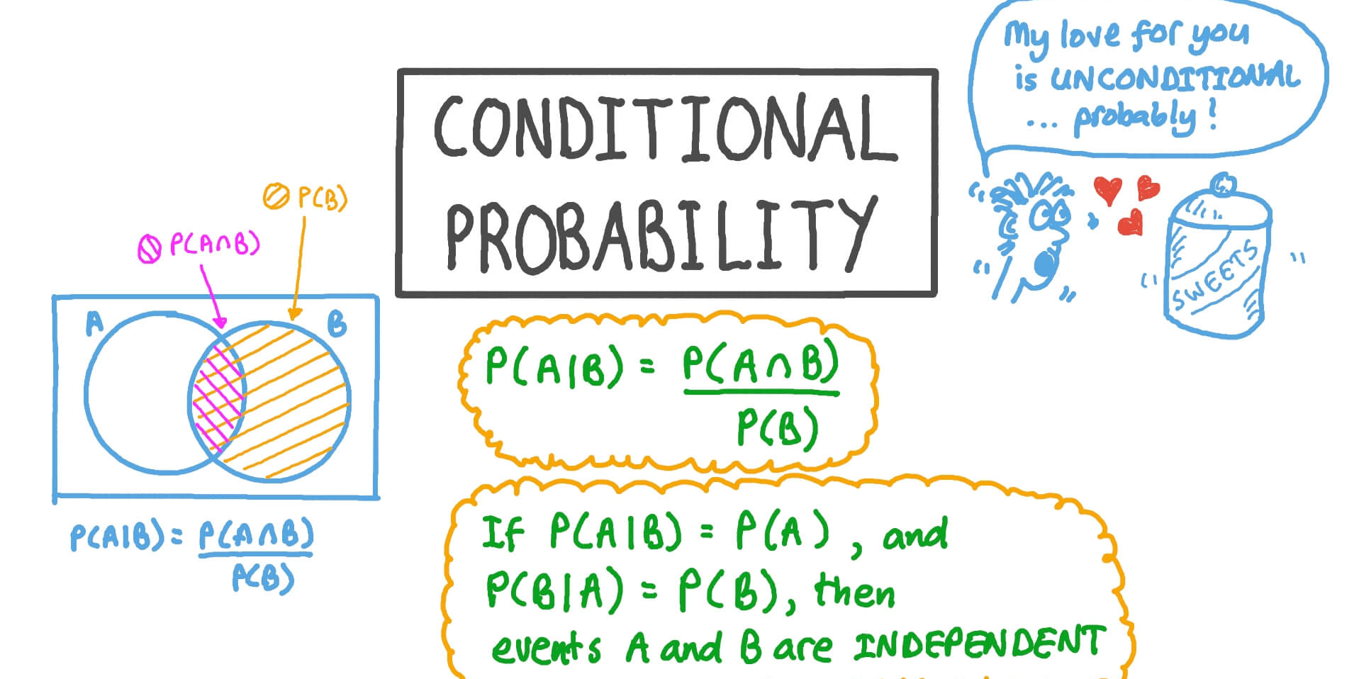
Bayes' Theorem

Bayes' theorem is a fundamental result in probability theory that relates conditional probabilities. It provides a way to update the probability of an event based on new evidence and is given by:

\[P(A|B) = \frac{P(B|A) \times P(A)}{P(B)}\]

Bayes' theorem is widely used in various fields, including statistics, machine learning, and decision theory, to make inferences and update beliefs based on observed data.

If you want to try applying these formulas, you can find example problems in the Study Bank at UpStudy.

History of Probability Research

The Beginnings in Gambling

Probability theory's roots can be traced to gambling and games of chance. Beginning in the 16th and 17th centuries, gamblers and mathematicians explored random events' rules with an aim of increasing their odds. This period witnessed early development of probability theory with notable contributions made by figures such as Gerolamo Cardano and Blaise Pascal, among many others.

16th and 17th Centuries

Foundational Work

Gerolamo Cardano was an Italian mathematician, physician, and gambler renowned for pioneering early work on probability theory. In his 1560 book Liber de Ludo Aleae (The Book on Games of Chance), written during that era and posthumously published in 1663, titled The Book on Games of Chance, he discussed basic probability principles as well as methods to calculate odds in various games.

Blaise Pascal and Pierre de Fermat, two prominent French mathematicians, made further strides forward in mathematics during the mid-17th century. Their correspondence on a gambling problem called Points (involving fair division of stakes in an interrupted game ) laid down a path toward modern probability theory through expected value models they developed—their work ultimately laid the basis of modern probability studies.

H4: Theory of Errors

In the late 17th century, error theory became an influential subject within probability studies. Pioneered by such luminaries as Isaac Newton and Edmond Halley, it dealt with measuring errors as well as their distribution across measurements. Error theory played an essential part in creating statistical methods as well as applying probability to scientific observations.

19th and 20th Centuries

Method of Least Squares

In the 19th century, probability theory and statistics saw significant advances. Carl Friedrich Gauss (a German mathematician) introduced Carl's Least Squares method, which minimizes the sum of squares differences between observed and predicted values by applying Carl Friedrich Gauss' method of least squares, an important technique related to the theory of errors that later became a core part of statistical analysis and regression models.

Central Limit Theorem

The Central Limit Theorem (CLT), one of the key results in probability theory, was first developed between 1881 and 1920. According to this theorem, when taken together, multiple independent, randomly distributed random variables approach normal distribution at any level in their sum total distribution—regardless of how they were originally distributed—their sum (or average distribution) will eventually resemble this normal curve distribution resulting from statistical inference or analysis of random phenomena. It has wide-reaching applications.

Probability theory continued its progress during the 20th century thanks to contributions by mathematicians like Andrey Kolmogorov, who formalized its axiomatic foundations, and Paul Lévy, who made significant advances in stochastic processes research. Such developments cemented probability theory's place as an essential branch of mathematics with numerous applications in science, engineering, economics, and beyond.

Applications of Probability

Applications in Theoretical Sciences

Probability theory plays a crucial role in various theoretical sciences, providing the mathematical framework to model and analyze random phenomena.

Physics

Probability plays an indispensable role in understanding and predicting the behavior of systems at both macroscopic and microscopic levels of scale, including quantum mechanics which heavily relies on probabilities in order to describe particle behavior; its probabilistic nature can be captured within its wave function which describes probabilities associated with finding particles in various states of motion.

Biomedical Sciences

Probability can be used in biomedical sciences to study treatment effectiveness, disease spread, and genetic inheritance patterns. Clinical trials relying heavily on statistical methods derived from probability theory employ statistical techniques derived from probability theory for efficacy testing of new medications, while epidemiologists utilize probability models to track transmission dynamics of infectious disease transmission dynamics as well as predict outbreaks.

Computer Science

Probability is at the core of computer science, particularly in areas such as machine learning, artificial intelligence, and algorithms. Probabilistic models and methods are employed in developing algorithms capable of learning from data sets, making predictions with limited information, or handling uncertainty effectively. Bayesian networks—an instance of a probabilistic graphical model used for reasoning under uncertainty—serve this function effectively.

Social Sciences

Probability has become an indispensable tool of social sciences research to study human behavior, social interactions, and economic phenomena. Surveys, experiments, and observational studies all utilize statistical techniques derived from probability theory in order to analyze data about populations, while economists make use of probability models in studying market behavior such as risk and decision-making under uncertainty.

Applications in Real Life

Probability isn't simply an abstract concept: its applications extend well into everyday life.

Applications in Meteorology

Probability has long been used in meteorology to forecast weather conditions and extreme events like hurricanes and tornadoes, using probabilistic models that analyze historical weather data, generate forecasts that reflect atmospheric processes' uncertainty, and assist individuals and organizations in making informed decisions regarding activities or safety measures.

Applications in Finance

Probability plays an essential role in finance by helping to model and mitigate risk, analyze investment opportunities, and price financial derivatives. Probabilistic models like Black-Scholes are used to estimate fair values of options and other financial instruments while risk managers employ VaR analysis methods such as Value at Risk to measure portfolio exposures to risk and assess and reduce them accordingly.

Games and Gambling

Probability plays an integral part in gaming and gambling, where it's used to calculate odds, create strategies, and evaluate game fairness. Understanding probability helps players make informed decisions and manage risks more effectively; casinos use probability models to create games that are both enjoyable and profitable.

Reference:

1. https://en.wikipedia.org/wiki/Probability

2. https://en.wikipedia.org/wiki/Probability_theory