What is a Probability Density Function?

Understanding the Basics of Probability Density Functions

Why Do We Need PDFs?

Probability density functions (PDFs) are vital tools in probabilistic analysis as they enable us to represent the behavior of continuous random variables. While discrete random variables use probability mass functions (PMFs) to assign probabilities at specific points, continuous random variables cannot have non-zero probabilities at specific locations, and therefore, probabilities must be distributed over intervals - this distribution process is something PDFs describe by assigning probabilistic densities at every possible value.

Consider measuring height among people in a population. Height is a continuous variable--its values range between 160.4 cm and 164.425 cm--thus creating the need for using probabilities density functions to describe certain ranges. A PDF could tell us, for instance, that individuals around 170 cm have higher probabilities compared with 180 cm even though exact measurements like 171.038 cm may not hold exact probabilities.

Discrete distributions, such as rolling a fair six-sided die, operate differently. In this case, individual outcomes have distinct probabilities (e.g., \(P(X = 3) = \frac{1}{6}\)). PDFs generalize probability calculations to intervals for continuous variables, making them invaluable in fields like statistics, finance, and scientific data analysis.

Key Definitions of PDFs

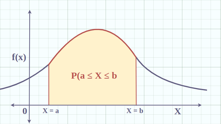
A probability density function represents probability per unit length. For a random variable \(X\), its PDF \(f_X(x)\) provides a way to calculate probabilities over intervals. The probability that \(X\) falls within an interval \([a, b]\) is given by:

\(P(a \leq X \leq b) = \int_a^b f_X(x) dx\)

The value of \(f_X(x)\) at a point \(x\) itself does not represent probability but rather the density of probability around \(x\). Mathematically, it is defined as the limiting ratio:

\(f_X(x) = \lim_{\Delta \to 0+} \frac{P(x < X \leq x + \Delta)}{\Delta}\)

Thus, PDFs are fundamental in describing how probabilities are distributed for continuous variables.

PDFs and Analogies in Real Life

PDFs may be easier to comprehend if they're seen as similar to mass density in physics; just as mass is distributed over an area (for instance, grams per centimeter), probability distribution occurs across values in random variables. If the density at a certain point on a mass distribution curve is high, this indicates that a lot of mass exists in that region. In the same way, a high value of a PDF indicates a high concentration of probability in a specific range. The total mass corresponds to a total probability of 1, matching the core requirement of a PDF.

The Mathematical Foundations of PDFs

The Formal Definition of a PDF

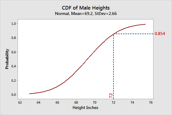
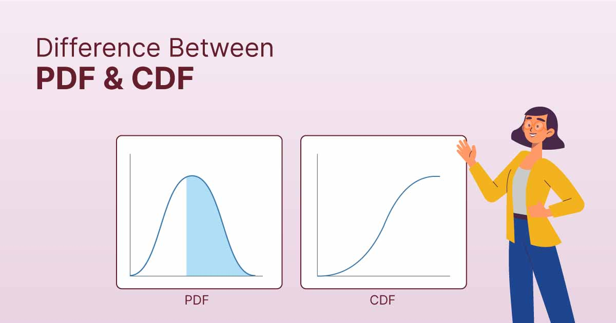
A probability density function is formally defined in relation to the cumulative distribution function (CDF) of a random variable \(X\). The CDF \(F_X(x)\) provides the probability that \(X\) is less than or equal to \(x\), and the PDF is derived as the derivative of the CDF:

\(f_X(x) = \frac{dF_X(x)}{dx}\)

Likewise, the CDF can be obtained by integrating the PDF:

\(F_X(x) = \int_{-\infty}^x f_X(u) du\)

This relationship between a PDF and a CDF is pivotal for understanding how probabilities are distributed. For example, if you sum all probabilities up to a certain value \(x\), the CDF captures this cumulative probability, while the PDF represents the rate of change at that point.

Properties of PDFs

Core Properties

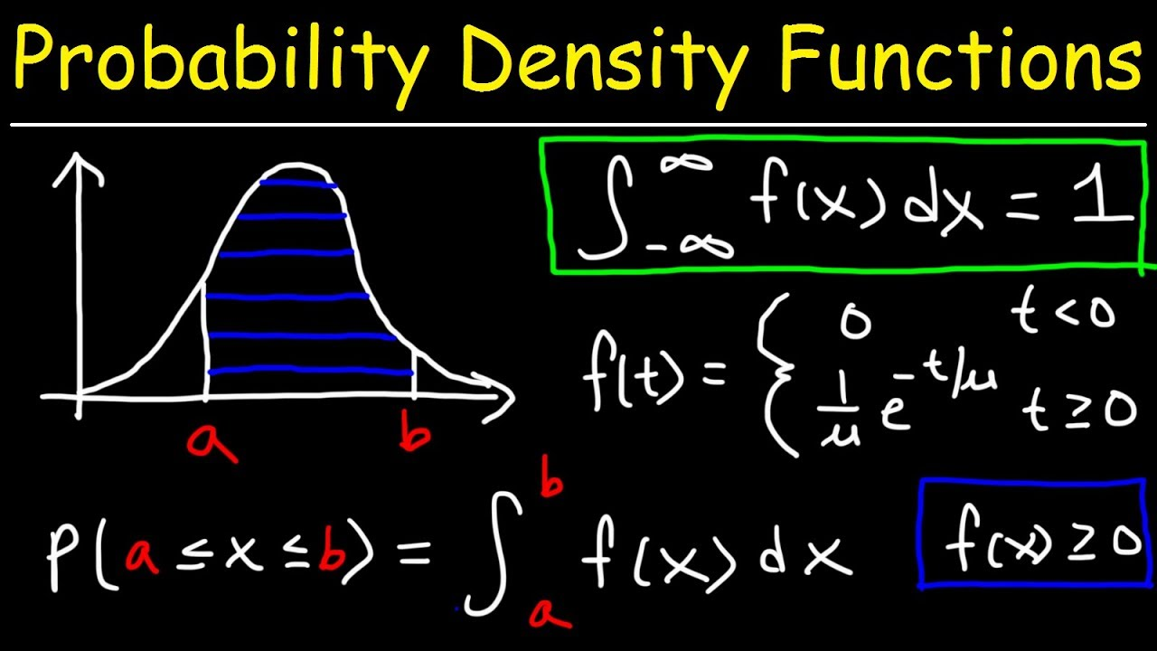
1. Non-Negativity: The PDF \(f_X(x)\) is always greater than or equal to 0 for all values of \(x\):

\(f_X(x) \geq 0\)

This ensures that probabilities or densities cannot be negative.

2. Normalization: The area under the entire curve of the PDF equals 1:

\(\int_{-\infty}^{+\infty} f_X(x) dx = 1\)

This property guarantees that the total probability over all possible values of \(X\) is equal to 1, reflecting the foundational principles of probability theory.

3. Probability Interpretation for Intervals: The probability of \(X\) falling within an interval \([a, b]\) is given by:

\(P(a \leq X \leq b) = \int_a^b f_X(x) dx\)

This allows PDFs to be used for practical probability calculations.

Support and Constraints

A PDF is defined over the support of a random variable, which is the set of all possible values where \(f_X(x) > 0\). For example, if a variable only takes positive values, its PDF might have a support of \([0, \infty)\).

Understanding PDF Properties with Examples

To illustrate the properties of PDFs, consider the uniform distribution for \(X\) over \([0, 1]\). The PDF is constant, \(f_X(x) = 1\), across this interval. There's no probability outside this range because \(f_X(x) = 0\) otherwise. Calculating the total area under this curve confirms it integrates to 1:

\(\int_0^1 1 \, dx = 1\)

Similarly, computing \(P(0.2 \leq X \leq 0.8)\) requires an integral over the interval:

\(P(0.2 \leq X \leq 0.8) = \int_{0.2}^{0.8} 1 \, dx = 0.8 - 0.2 = 0.6\)

These calculations directly highlight how the fundamental properties of PDFs apply in practice.

The Relationship Between PDFs and CDFs

From CDF to PDF

The relationship between PDFs and cumulative distribution functions (CDFs) reflects the deeper mathematical structure of probability. A CDF \(F_X(x)\) characterizes the probability that the random variable \(X\) takes a value less than or equal to \(x\):

\(F_X(x) = P(X \leq x)\)

Deriving the PDF from the CDF involves differentiation:

\(f_X(x) = \frac{dF_X(x)}{dx}\)

For example, consider a uniform random variable \(X\) over \([0, 1]\) with the CDF:

\(F_X(x) = \begin{cases} 0, & x < 0 \\ x, & 0 \leq x \leq 1 \\ 1, & x > 1 \end{cases}\)

Differentiating this yields the PDF:

\(f_X(x) = \begin{cases} 1, & 0 \leq x \leq 1 \\ 0, & \text{otherwise.} \end{cases}\)

This represents a constant PDF over \([0, 1]\).

From PDF to CDF

Conversely, we can reconstruct the CDF by integrating the PDF:

\(F_X(x) = \int_{-\infty}^x f_X(u) du\)

As an example, take the PDF of an exponential distribution:

\(f_X(x) = \begin{cases} \lambda e^{-\lambda x}, & x \geq 0 \\ 0, & x < 0 \end{cases}\)

The CDF is obtained via integration:

\(F_X(x) = \begin{cases} 1 - e^{-\lambda x}, & x \geq 0 \\ 0, & x < 0 \end{cases}\)

This bidirectional relationship highlights how PDFs and CDFs complement each other in representing continuous probabilities.

Interpreting PDFs: What Does It Tell Us?

The Meaning of Probability Density at a Point

The interpretation of probability density is central to understanding PDFs. Contrary to discrete probability functions that assign non-zero probabilities to individual outcomes, PDFs only describe densities, not absolute probabilities, at specific points. For a continuous random variable \(X\), the probability that \(X\) takes an exact value \(x\) is always zero:

\(P(X = x) = 0, \, \text{for any } x\)

Instead, the value of the PDF \(f_X(x)\) at a point \(x\) reflects the relative likelihood of finding \(X\) near that value. For example, if \(f_X(x_1) > f_X(x_2)\), the areas around \(x_1\) are more likely to contain observations compared to \(x_2\).

To calculate probabilities or likelihoods, one must evaluate the total probability over an interval by integrating the PDF:

\(P(a \leq X \leq b) = \int_a^b f_X(x) dx\)

Thus, \(f_X(x)\) is not a probability but instead measures how probability is distributed across values of \(X\).

Visualizing PDFs for Better Intuition

Imagine zooming in on a PDF graph at a specific point \(x\) and examining a small interval \([x, x + \delta]\). The approximate probability of \(X\) being in this interval can be calculated using the density function:

\(P(X \in [x, x + \delta]) \approx f_X(x) \cdot \delta\)

For instance, consider a normal distribution of people's weights. The PDF may peak near a mean weight like 70 kg, suggesting the highest density of probabilities is concentrated here.

General Use Cases of PDF Interpretation

PDFs offer more than mathematical benefits; their real-world applications extend well beyond pure mathematics. For instance, when used to ensure quality control on manufacturing parts, PDFs provide engineers with a way to monitor dimensions that fall into acceptable tolerance limits while effectively pinpointing areas with increased likelihood and variability.

Example Applications of PDFs in Real-World Scenarios

Applications in Statistics and Data Science

PDFs play an integral part in statistical inferential analysis and likelihood estimation, including model building. When fitting normal distributions to data such as test scores, PDFs help deduce probabilities associated with observed values under specific assumptions; for instance, fitting one allows researchers to calculate how many students scored above or within certain threshold ranges on test scores.

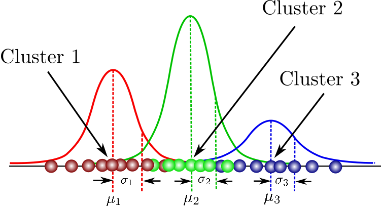
Machine learning applications also utilize PDFs as part of their approach to modeling uncertainty, optimizing classification boundaries and simulating probabilistic behaviors, such as those found in Gaussian Mixture Models (GMMs).

Engineering and Scientific Modelling Applications

PDFs play an essential role in engineering tasks related to reliability analysis. For instance, reliability engineering often follows an exponential distribution that the PDF helps predict probabilities of failure within particular time intervals. Furthermore, PDFs play a vital part in driving sensor-based systems where traffic flow or signal intensities follow specific probability distributions.

Scientific researchers frequently utilize PDFs in scientific research, especially to model particle behavior in physics. Quantum particles display probability densities; using PDFs allows scientists to assess the probability that certain positions or momentums exist for any particular particle.

Design and Optimizations in Real-world Systems

PDFs are effectively applied in financial risk modeling to estimate the likelihood of extreme drawdowns, weather forecasting by modeling temperature variations and even in gaming to ensure fair distributions of rewards or outcomes. For instance, in designing loot-drop mechanisms in video games, balanced underlying distribution functions (represented by PDFs) ensure fair and engaging gameplay for users.

Misunderstandings About PDFs and Clarifications

Misconceiving PDFs as Actual Probabilities

A common misconception about PDFs is mistaking the value \(f_X(x)\) for the probability that a random variable \(X\) equals \(x\). This misunderstanding arises because people tend to confuse the density at a single point with a discrete probability. For continuous random variables, however:

\(P(X = x) = 0\)

Instead of providing probabilities for specific points, PDFs describe how that probability is spread out across the range of possible values.

Zero-probability events Do Not Mean Impossibility

An important clarification is that while \(P(X = x) = 0\) for any continuous variable, this does not mean the occurrence of \(X = x\) is impossible. It simply reflects the fact that the chance of randomly landing on an exact value in a theoretically infi\(P(X = x) = 0\)sured with infinite precision. However, the exact height, like 170.0000... cm, has zero individual probability. Instead, we calculate probabilities over realistic intervals, such as \(P(169.9 \leq X \leq 170.1)\).

By understanding this nuance, one can better interpret and utilize PDFs in a variety of contexts without falling into common conceptual pitfalls.

Leveraging PDFs to Understand Data Distributions

Analyzing Probability Densities in Data

Probability density functions (PDFs) provide powerful ways of exploring data distribution characteristics. By observing its shape, one can gain key insight into the spread, central tendency, and variability of any random variable.

Comparing the PDF of a uniform distribution and normal distribution reveals significant variations in data distribution. A uniform distribution depicts equal likelihood across values, while a normal distribution concentrates probabilities near its center before tapering off into tails.

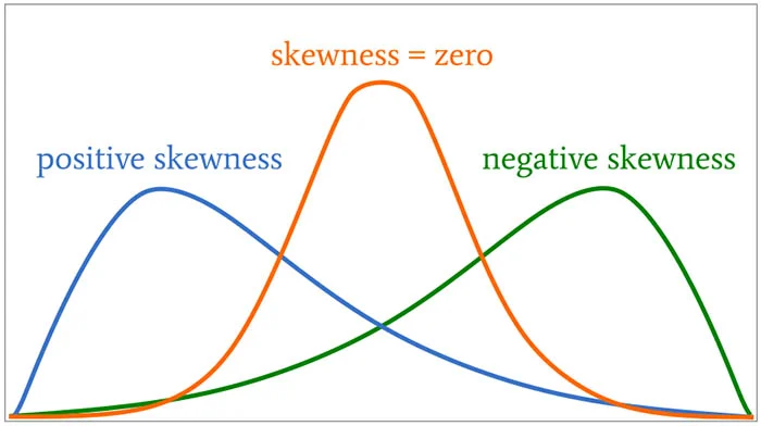
PDFs also enable researchers to detect skewness and kurtosis; such distributions could indicate asymmetric tendencies within data, while kurtosis indicates whether probabilities cluster nearer to or further from their average.

Visualizing PDFs as a Data Analysis Tool

Imagine a PDF graph similar to a topographical map: its peak indicates regions where data points (or probabilities) accumulate more frequently, while valleys indicate sparser areas. By overlaying multiple PDFs, researchers can compare distributions from various datasets - for instance, income distribution across demographic groups - revealing patterns, trends, or anomalies that would otherwise remain hidden from view.

Visualizing PDFs in conjunction with histograms or kernel density estimates (KDEs) enables practitioners to transition from abstract mathematical descriptions of data sets to more practical, accessible data insights.

Common Types of Probability Distributions and Their PDFs

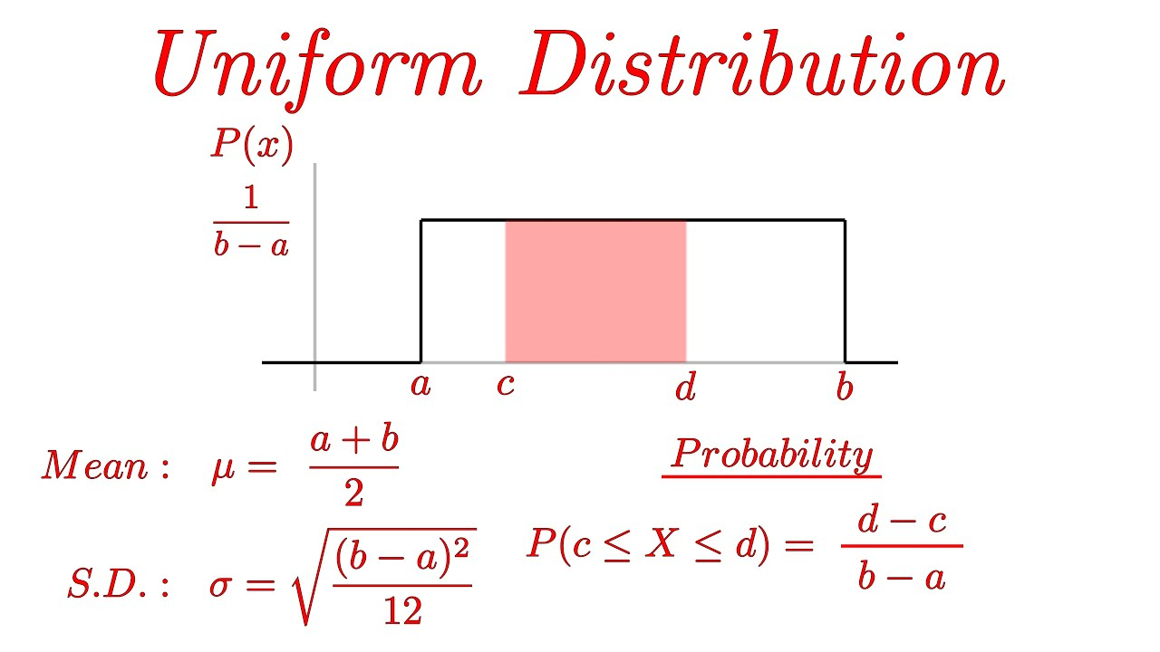
Uniform Distribution

The uniform distribution represents a random variable with equal probabilities across an interval \([a, b]\). Its PDF is given by:

\(f_X(x) = \begin{cases} \frac{1}{b - a}, & \text{if } a \leq x \leq b \\ 0, & \text{otherwise} \end{cases}\)

For example, rolling a fair die can be modeled as a discrete analog to a uniform distribution with equal probabilities across outcomes.

Normal Distribution

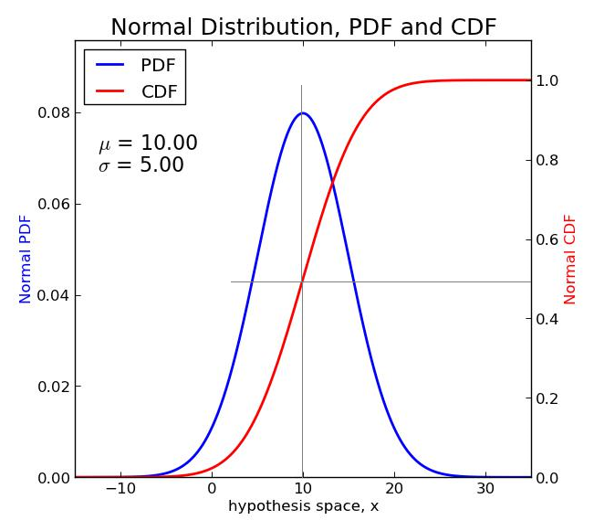
The normal (Gaussian) distribution, described by the bell-shaped curve, is one of the most widely used distributions. Its PDF is:

\(f_X(x) = \frac{1}{\sqrt{2\pi\sigma^2}} e^{-(x - \mu)^2 / (2\sigma^2)}\)

Here, \(\mu\) is the mean and \(\sigma^2\) is the variance. This distribution is foundational in statistics due to the central limit theorem, which states that sample means from any population will tend to follow a normal distribution.

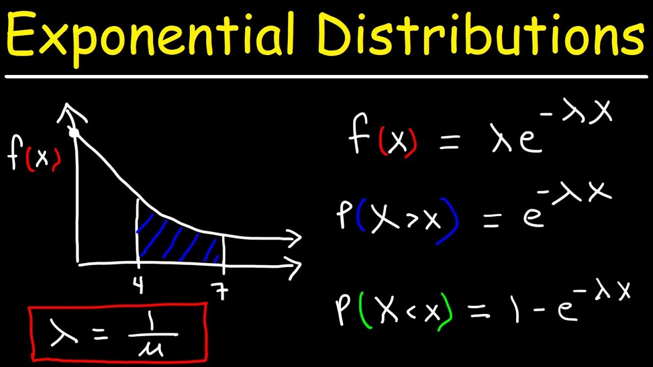
Exponential Distribution

The exponential distribution is widely used in reliability and lifespan modeling. Its PDF is:

\(f_X(x) = \begin{cases} \lambda e^{-\lambda x}, & \text{if } x \geq 0 \\ 0, & \text{otherwise} \end{cases}\)

Here, \(\lambda\) determines the rate of decay, reflecting the likelihood of an event occurring in a fixed time frame—useful in scenarios like machinery failures or queuing systems.

Conclusion

Probability density functions (PDFs) form an essential foundation of continuous probability theory, providing the bridge from abstract mathematical ideas to real world applications. By understanding their properties, relationships to cumulative distribution functions (CDFs), and practical implications we gain tools for analyzing datasets, modeling uncertainties and making predictions.

PDFs offer great flexibility across engineering, statistics, and data science applications ranging from signal processing to financial risk evaluation. By understanding their foundational principles - such as normalization and density interpretation - users can utilize PDFs effectively and utilize randomness with confidence - making PDFs indispensable tools in studying probabilistic phenomena.

Reference:

https://medium.com/towards-data-science/kernel-density-estimation-explained-step-by-step-7cc5b5bc4517 

https://libanswers.lib.miamioh.edu/stats-faq/faq/343628

https://en.wikipedia.org/wiki/Exponential_distribution